bland c++
目录(Table of contents)
Why using the Bland-Altman plot
为什么要使用Bland-Altman图
The used data
使用的数据
How the Bland-Altman plot is built
布兰德·奥特曼图的构建方式
How to interpret the Bland-Altman plot for A/B test
如何解释A / B测试的Bland-Altman图
Conclusion
结论
为什么要使用Bland-Altman图(Why use the Bland-Altman plot)
The Bland-Altman plot comes from the medical industry in order to compare the measure for two instruments. The first objective of John Martin Bland & Douglas Altman was to answer this question :
Bland-Altman图来自医疗行业,目的是比较两种仪器的测量值。 John Martin Bland和Douglas Altman的首要目标是回答这个问题:
Do the two methods of measurement agree sufficiently closely ? — D. G. ALTMAN and J. M. BLAND [1]
两种测量方法是否足够接近? — DG ALTMAN和JM BLAND [1]
If it is the case, it means that if you have two instruments where one is the state of the art at a high cost and the second is 10 times cheaper, do the results obtained by the cheapest method are comparable to the reference and could it be replaced with a sufficient accuracy? For example, does the heart rate provided by a $20 connected watch is sufficiently accurate as the result of an electrocardiogram ? The second objective was to produce a method where the results are easily understandable to non-statisticians.
如果是这样,则意味着如果您有两台仪器,其中一台是最新技术,价格高昂,而另一台则便宜10倍,那么用最便宜的方法获得的结果是否可与参考相比?被足够的精度所取代? 例如,作为心电图检查的结果,一块价值20美元的手表所提供的心率是否足够准确? 第二个目标是提供一种方法,使非统计学家容易理解结果。
In analytics, A/B testing (as well known as Champion-Challenger) is a common methodology of test to compare the results of a new action / a new treatment / a new design / … on population_A to population_B having the current action. Once we have the test’s results, they have to be analysed and presented to a decisional team mostly composed of non-statisticians. That is why the Bland-Altman plot is relevant because it will compare the results of the A/B test on one plot with all of the statistical measures displayed in an understandable way.
在分析中,A / B测试(即众所周知的Champion-Challenger)是一种常见的测试方法,用于比较针对种群_A的新操作/新处理/新设计/…的结果与具有当前操作的种群_B的结果。 一旦获得测试结果,就必须对其进行分析,并提交给主要由非统计人员组成的决策团队。 这就是为什么Bland-Altman图具有相关性的原因,因为它将以一种易于理解的方式将A / B测试在一个图上的结果与所有统计量进行比较。
In their paper, they also showed why the correlation coefficient, the statistical test of mean comparison and the regression are inappropriate to decide on the agreement of two measures which would be in our A/B testing case to decide on the power of the challenger compared to the one of the champion.
在他们的论文中,他们还表明了为什么相关系数,均值比较的统计检验和回归分析不适合决定两种方法的一致性,而这在我们的A / B测试案例中就无法确定所比较挑战者的能力给冠军之一。
使用的数据 (The used data)
For this article I will use a dataset available on Kaggle (coming from a DataCamp project) called “Mobile Games A/B Testing with Cookie Cats”. The link are in the references part [2].
在本文中,我将使用Kaggle(来自DataCamp项目)上可用的数据集,称为“使用Cookie Cats进行Mobile Games A / B测试”。 链接在参考部分[2]中。
Cookie Cats is a popular mobile puzzle game where as a player progress the levels, he will encounter “gates” that will force him to wait for some time before continuing to play or to make a purchase. In such an industry the retention is one of the key metrics and the team in charge of the game would see the impact if the first gate was moved from level 30 to level 40 on the retention at 7 days. To see the behavior of such a move they did an A/B test and they provided us the dataset of these results. We will see how the Bland-Altman plot will answer the following question : “How to analyze the A/B results on the level of retention at 7 days when the waiting time passes from the level 30 to the level 40 ?”
Cookie Cats是一款流行的移动益智游戏,随着玩家逐步升级关卡,他将遇到“门”,这将迫使他等待一段时间才能继续玩或进行购买。 在这样的行业中,保留率是关键指标之一,负责游戏的团队会发现,如果第一个门在7天时从30级升至40级,则会对保留率产生影响。 为了查看此举的行为,他们进行了A / B测试,并向我们提供了这些结果的数据集。 我们将看到Bland-Altman图将如何回答以下问题:“当等待时间从30级变为40级时,如何分析7天保留率的A / B结果?”
The dataset is composed of 90.189 rows where we have the player’s unique id, the A/B test’s version (waiting time at gate_30 / gate_40), the game rounds’ sum, retention_1 is a boolean saying if the player came back on the next day and retention_7 is a boolean saying if the player came back after 7 days. In order to have the relevant data to answer our question, it is necessary to do some cleaning. I will only keep the client having a retention_1 = True (because if retention_1=False, retention_7 is False as well), a number of game rounds ≥ 30 (because if they don’t go until 30, they will not be impacted by the gate) and a number of game rounds < 170 (because if we consider the duration of a game = 5 minutes, if a player plays 2 hours per day during 7 day he will play 120*7/5 = 168 games. A higher number would be considered as an anormal usage). After this filter, the dataset is composed of 20.471 rows as Figure1 below. Moreover, the dataset is equally balanced between gate_30 & gate_40.
数据集由90.189行组成,其中有玩家的唯一ID,A / B测试的版本(等待时间在gate_30 / gate_40),游戏回合的总和,retention_1是一个布尔值,表示玩家是否在第二天回来保留值[7]是布尔值,表示玩家是否在7天后回来。 为了获得相关数据来回答我们的问题,有必要进行一些清洁。 我只会让客户保持值_1 = True(因为如果retention_1 = False,retention_7也为False),游戏回合数≥30(因为如果直到30时才回合,则不会受到影响)门数)和小于170的游戏回合数(因为如果我们考虑游戏的持续时间= 5分钟,则如果玩家在7天中每天玩2个小时,他将玩120 * 7/5 = 168场游戏。将被视为正常使用)。 经过此过滤器后,数据集由20.471行组成,如下图1所示。 此外,数据集在gate_30和gate_40之间均等地平衡。
Figure1. CookieCats dataset 图1。 CookieCats数据集如何建立Bland-Altman图(How is built the Bland-Altman plot)
We will see on this section how to adapt the original Bland-Altman plot in order to apply it to an A/B test. First of all I am going to explain how is the plot built in its original version [1], [2] and then, I will explain how to build it with our A/B tests’ data.
我们将在本节中看到如何适应原始的Bland-Altman图,以将其应用于A / B测试。 首先,我将解释如何在原始版本[1],[2]中构建图表,然后,将解释如何使用A / B测试数据构建图表。
Due that the original Bland-Altman plot compare the measurement of 2 instruments, they have the same length by design. For example, with the heart rate measurement between the $20 connect watch and the electrocardiogram, the measure are taken on the same time with the same conditions which lead to have the same number of measurement for the 2 methods. So we can represent each dataset’s row as an experience like on the example in the Figure2 below.
由于原始的Bland-Altman图比较了两种仪器的测量结果,因此它们在设计上具有相同的长度。 例如,在$ 20 Connect手表和心电图之间进行心率测量时,在相同条件下同时进行测量,导致这两种方法的测量次数相同。 因此,我们可以将每个数据集的行表示为一种体验,就像下面的图2中的示例一样。
Figure2. Instrument measure per experience 图2。 根据经验衡量This is where we encounter the first “pain point”. An A/B test is considered as an unique experience while as we see above, we need several experiences in order to build the plot. To bypass this limitation we will create from the A/B test several bootstrapped samples having both the same & different length.
这是我们遇到的第一个“痛点”。 A / B测试被认为是独特的体验,而正如我们上面所看到的,我们需要一些经验来构建图。 为了绕过此限制,我们将从A / B测试中创建几个长度相同且长度不同的自举样本。
We generate 300 non-unique random integers between 200 and 1.000. These integers will represent the length of each bootstrapped sample and in order to benefit the bootstrap’s statistical properties, each non-unique random integer is duplicated 50 times. These numbers are used in order to have a sample diversity but it is arbitrary and the length depends from the size of the original dataset. These 15.000 (300*50) bootstrapped samples having a length between 200 and 2.000 are obtained by a random sampling with a replacement from the original dataset and they are concatenated together. It can be represented as the Figure3.
我们生成200到1.000之间的300个非唯一随机整数。 这些整数将代表每个自举样本的长度,并且为了受益于引导程序的统计属性,每个非唯一随机整数均重复50次。 使用这些数字是为了使样本具有多样性,但它是任意的,其长度取决于原始数据集的大小。 这些长度为200到2.000之间的15.000(300 * 50)个自举样本是通过从原始数据集中进行替换的随机抽样获得的,并将它们串联在一起。 它可以表示为图3。
The following code creates the bootstrapped dataset from the original data (be careful, it can takes time because the bootstrapped dataset has a length of 9.184.350 rows {by changing the random_state, we would have in average (((200+1.000)/2)*300*50 = 9.000.000 rows}).
以下代码根据原始数据创建自举数据集(请注意,这可能会花费一些时间,因为自举数据集的长度为9.184.350行{通过更改random_state,我们平均可以得到((((200 + 1.000)/ 2)* 300 * 50 = 9.000.000行} )。
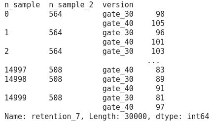
Then, we group by n_sample (the id of each 15.000 bootstrapped sample), n_sample_2 (the length of each bootstrapped sample) and version in order to have the sum of player’s retention at 7 days per gates as in Figure 4.
然后,我们将n_sample(每个15.000自举样本的ID),n_sample_2(每个自举样本的长度)和版本进行分组,以使每个门的玩家保留天数总计为7天,如图4所示。
Figure4. Bootstrapped dataset after groupby 图4。 分组后引导数据集We can read this output as: the bootstrapped sample n°0/14.999 is composed of 564 rows where 98 players are still playing at 7 days with a waiting time at gate_30 while 105 players are still playing at 7 days with a waiting time at gate_40.
我们可以将输出读取为:引导样本n°0 / 14.999由564行组成,其中98个玩家在7天仍在玩游戏,等待时间在gate_30,而105个玩家仍在7天在玩游戏,等待时间在gate_40 。
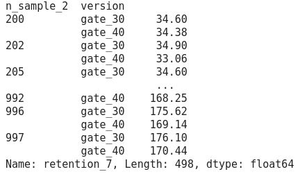
Then, we use a statistical property of the boostrap saying that the mean of a bootstrap sample is a good estimator of the true mean of a distribution. We make a group by n_sample_2 and version in order to have for each unique sample’s length the average number of player’s retention at 7 days per gates as in Figure 5.
然后,我们使用boostrap的统计性质,即自举样本的均值是分布真实均值的良好估计。 我们按n_sample_2和版本进行分组,以便针对每个唯一样本的长度,每个门在7天的平均玩家保留数如图5所示。
Figure5. Average number of players still playing at 7 days for each unique sample length and per gates 图5。 每个唯一的样本长度和每个门,仍在玩7天的平均玩家数量We can read this output as: when the sample has 200 rows there are in average 34.60 players who are still playing at 7 days with a waiting time at gate_30 while 34.38 players who are still playing at 7 days with a waiting time at gate_40.
我们可以将输出读取为:当样本有200行时,平均有34.60名玩家仍在7天的比赛中等待时间在gate_30处,而仍有34.38名玩家仍在7天的比赛中等待时间在gate_40处。
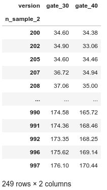
Then we unstack the database in order to have the dataset in a clearer format as the Figure6.
然后我们对数据库进行拆栈,以使数据集的格式更加清晰,如图6所示。
Figure6. Unstacked version of the dataset 图6。 数据集的未堆叠版本At this stage we have all the necessary information in order to build the Bland-Altman plot and the representation of the dataset is the same as in the Figure2 above.
在此阶段,我们拥有所有必要的信息以构建Bland-Altman图,并且数据集的表示与上图2相同。
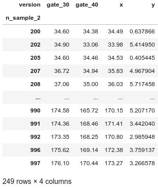
The Bland-Altman plot is composed of 2 axis. The x axis is the average of the two methods to compare. So it is for each row: (gate_30i + gate_40i) / 2 ||| The y axis is the difference between method A and method B. So it is for each row: (gate_30i - gate_40i) ||| And here is the second “pain point” we have. By keeping the y axis as it is, the increase of the samples’ size will increase the differences’ variability. As a result, the statistical measure we will obtain later will be over-weighted by the biggest samples. To bypass this limitation, we will represent the y axis in percentage [3]. To do it, the calculation of y is for each row: ((gate_30i - gate_40i)*100 / (( gate_30i + gate_40i)/2) ||| The dataset looks like Figure7.
Bland-Altman图由2轴组成。 x轴是两种比较方法的平均值。 每一行都是这样:(gate_30i + gate_40i)/ 2 ||| y轴是方法A和方法B之间的差。 每一行都是这样:(gate_30i-gate_40i)||| 这是我们的第二个“痛点”。 通过保持y轴不变,样本大小的增加将增加差异的变异性。 结果,我们稍后将获得的统计量将被最大样本所加权。 为了绕过此限制,我们将以百分比[3]表示y轴。 为此,对每一行进行y的计算:((gate_30i-gate_40i)* 100 /(((gate_30i + gate_40i)/ 2)|||数据集如图7所示。
Figure7. x & y axis 图7。 x&y轴We have to check that the y axis is normally distributed in order to trust the confidence interval who will be displayed. You can assess it by using the shapiro-wilk test or at least with an histogram. If the distribution is not Normal then you can do a transformation such as logarithmic transformation. In our case, I consider the distribution as Normal.
我们必须检查y轴是否正态分布,以便信任将显示谁的置信区间。 您可以使用shapiro-wilk检验或至少与直方图进行评估。 如果分布不是正态分布,则可以进行对数转换。 在我们的情况下,我认为该分布为正态分布。
Figure8. Histogram of the y axis 图8。 y轴的直方图The Bland-Altman is composed of 3 lines (see Figure9):
Bland-Altman由3条线组成(请参见图9):
the average values of y
y的平均值
the y’s upper bound of the confidence interval (here at 95% given the 1.96)
y的置信区间上限(此处为1.96的95%)
the y’s lower bound of the confidence interval (at 95%)
y的置信区间下限(95%)
We put all together, the package pyCompare allows to draw the Bland-Altman plot on a very easy way without having to build db[‘y’]:
我们放在一起,包pyCompare允许以非常简单的方式绘制Bland-Altman图,而无需构建db ['y'] :
It takes first the method A (the champion) and then the method B (the challenger). Then, if percentage = True, it will automatically do the calculus we made above. There are some other parameters we will discuss later.
它首先采用方法A(冠军),然后采用方法B(挑战者)。 然后,如果percent = True ,它将自动执行我们上面进行的演算。 我们稍后还会讨论其他一些参数。
如何为A / B测试解释Bland-Altman图 (How to interpret the Bland-Altman plot for the A/B test)
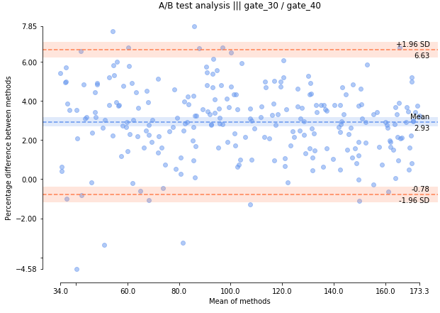
Here we are ! Here is the figure of the Bland-Altman plot for the A/B testing generated by the code above:
我们来了 ! 这是上面的代码生成的A / B测试的Bland-Altman图的图:
Figure10. Bland-Altman plot applied for A/B test 图10。 Bland-Altman图应用于A / B测试First of all, the mean and the mean’s confidence interval (light blue stripe) are different than 0 (higher in our case). Which means that the level of retention (named bias in the original paper) of gate_30 and gate_40 are significantly different. Due that 2.93 > 0 it means that A > B < — > Champion > Challenger and as a result that a waiting period on gate_30 provides a bigger retention than a waiting period on gate_40.
首先,均值和均值的置信区间(浅蓝色条纹)不同于0(在我们的情况下较高)。 这意味着gate_30和gate_40的保留水平(在原始论文中称为偏见)显着不同。 由于2.93> 0,这意味着A> B <—>冠军>挑战者,结果是gate_30上的等待时间比gate_40上的等待时间更长。
The two salmon bars represent the confidence interval at 95% (named limit of agreement in the original paper) saying that we are convinced that 95% of the values will be between [-0.78% ; 6.63%]. In our exemple, this is very powerful because we can say that the retention of gate_30 will be almost always bigger than the one of gate_40.
两条鲑鱼条代表95%的置信区间(在原始论文中称为协议限制),表示我们确信95%的值将在[-0.78%之间; 6.63%] 。 在我们的例子中,这非常强大,因为可以说gate_30的保留几乎总是大于gate_40的保留。
As you can see, there are 2 values above the upper salmon stripe and 4 below the lower one, which is 6/300 = 0.02 < 0.05 so due that we are certain that 95% of the values are within the 2 boundaries, 5% can be above or below and in our case it represents 2% then it is perfectly normal ;)
如您所见,在上面的鲑鱼条上方有2个值,在下面的鲑鱼条下方有4个值,这是6/300 = 0.02 <0.05,因此我们可以确定95%的值在2个边界内,即5%可以高于或低于此值,在我们的示例中,它代表2%,那么这是完全正常的;)
In the pyCompare package there is the parameter limitOfAgreement who aims to change the boundaries of confidence. Here, a relevant question would be : “At which percentage can I be sure that the retention of gate_30 will be always bigger than the one of gate_40 ?” To answer this question, the lowest boundary has to be equal to 0, so we have to find the right value in order to have 0 as we can see in the code below which provide the Figure11:
在pyCompare包中,有一个参数limitOfAgreement旨在更改置信度边界。 在这里,一个相关的问题是:“我可以确保gate_30的保留率始终大于gate_40的保留率?” 要回答这个问题,最低边界必须等于0 ,所以我们必须找到正确的值才能有0,如下面提供Figure11的代码所示:
Figure11. Output when changing the limitOfAgreement’s parameter 图11。 更改limitOfAgreement参数时的输出We see that when limitOfAgreement = 1.55, the boundary is almost equal to 0. Then we have to check in the Normal distribution table the value at 1.55 which is 0.9394, so we are sure at ((1–0.9394)*2)*100 = 87.88% that the retention of gate_30 will always be bigger than the one of gate_40
我们看到,当limitOfAgreement = 1.55时,边界几乎等于0。然后我们必须在正态分布表中检查1.55处的值0.9394,因此我们可以确定((1–0.9394)* 2)* 100 = 87.88%,gate_30的保留总是大于gate_40的保留
A last point to add is that whatever the average value of the sample, they are uniformly represented on the plot which means that the interpretation we are making are generalized whatever the size of the sample is. Indeed if we had seen a kind of conic representation of the values we could have conclude that the size of the sample has an impact on the results so we cannot have a valid interpretation.
最后要补充的一点是,无论样本的平均值是多少,它们都在图表上统一表示,这意味着无论样本的大小如何,我们所做的解释都是通用的。 的确,如果我们看到值的一种圆锥形表示,我们可以得出结论,样本的大小会对结果产生影响,因此我们无法做出有效的解释。
结论 (Conclusion)
We saw why it can be relevant to use the Bland-Altman plot in order to have one view about the results of an A/B test on a simple plot, how to create the plot from an A/B test and how to interpret it. This only works in case of normality of the difference however it will be necessary to transform the data.
我们已经看到了为什么使用Bland-Altman图对一个简单图上的A / B测试结果有一个看法,如何从A / B测试创建图以及如何解释它的意义, 。 这仅在差异正常的情况下有效,但是有必要转换数据。
Moreover, I checked the App and the gates appears to be on gate_40 while we proved that the retention at 7 days was better at 30. In this case, it shows that the retention is maybe not the best metric to follow compared to the profitability !
此外,我检查了该应用程序,发现登机口位于gate_40上,而我们证明了7天的保留率要好于30天。在这种情况下,它表明与获利能力相比,保留率可能不是最佳的衡量标准!
翻译自: https://towardsdatascience.com/why-how-to-use-the-bland-altman-plot-for-a-b-testing-python-code-78712d28c362
bland c++


