逻辑回归（ROC、AUC、KS）-python实现-内含训练数据-测试数据

一、逻辑回归理论：关注代码上线

Hypothesis Function（假设函数）：1.0/(1+exp(-inX))

Cost Function（代价函数）：

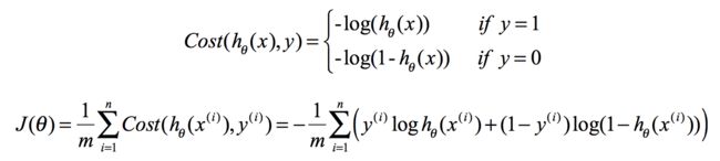
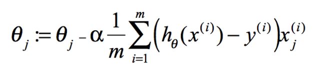
通过梯度下降法，求最小值。

weights(系数矩阵)=weights+alpha（固定值）*dataMatrix（特征指标）*error（真实值-预测值）
 

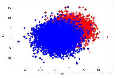
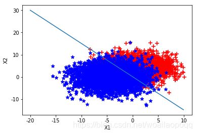
二、运行效果

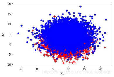
第一组：

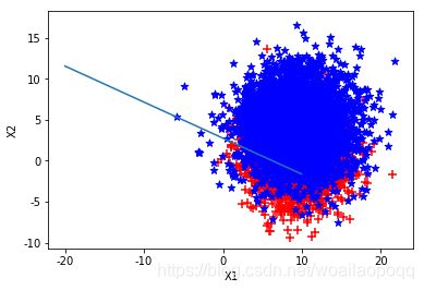
第二组：

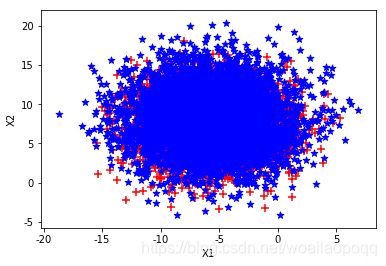
第三组：

三、python代码实现-梯度上升

import matplotlib.pyplot as plt
import numpy as np
from numpy import exp
from sklearn.metrics import confusion_matrix
from sklearn.metrics import roc_curve, auc
import pandas as pd
import matplotlib.pyplot as plt #导入图像库
import matplotlib
import seaborn as sns
import statsmodels.api as sm
from sklearn.metrics import roc_curve, auc
import math
from sklearn import metrics
from sklearn.datasets import make_classification
from sklearn.datasets import make_blobs
from sklearn.datasets import make_gaussian_quantiles
from sklearn.datasets import make_hastie_10_2
from sklearn.model_selection import train_test_split

#假设函数
def sigmoid(inX):
        return 1.0/(1+exp(-inX))
#获取预测Y值,系数为weights
def getValue(x,weights):
    return (weights[0, 0] - weights[1, 0] * x) / weights[2, 0]

    
#梯度上升方法求Cost Function   
def grad_descent(Xtrain,alpha,max_cycle):
     #划分训练数据，测试验证数据
    Y=Xtrain['y']
    #训练X
    X=Xtrain[['x0','x1','x2']]
    dataMatrix = np.mat(X).T  #(m,n)
    dataMatrix_sigmoid = np.mat(X)
    labelMat = np.mat(Y).T
    m,n = np.shape(X)
    weights = np.ones((n, 1))  #初始化回归系数（n, 1)
#    print('weights:\n',weights)
    
    
    
    for i in range(max_cycle):
        h = sigmoid(dataMatrix_sigmoid * weights)  #sigmoid 函数
        error=labelMat-h
        weights=weights+alpha*dataMatrix*error
    #绘制二分类图使用t_为Y=1，f_为Y=0
    t_x1=Xtrain.loc[(Xtrain['y']==1)]['x1']
    t_x2=Xtrain.loc[(Xtrain['y']==1)]['x2']
    
    f_x1=Xtrain.loc[(Xtrain['y']==0)]['x1']
    f_x2=Xtrain.loc[(Xtrain['y']==0)]['x2']
    fig = plt.figure()
    ax = fig.add_subplot(111)
    #y=1的点
    ax.scatter(f_x1,f_x2,marker='+',label='1',s=50,c='r')
    #y=0的点   
    ax.scatter(t_x1,t_x2,marker='*',label='1',s=50,c='b')
    """
    参数个数情况： np.arange()函数分为一个参数，两个参数，三个参数三种情况
    1）一个参数时，参数值为终点，起点取默认值0，步长取默认值1。
    2）两个参数时，第一个参数为起点，第二个参数为终点，步长取默认值1。
    3）三个参数时，第一个参数为起点，第二个参数为终点，第三个参数为步长。其中步长支持小数
    """
#    print('weights:\n',weights)
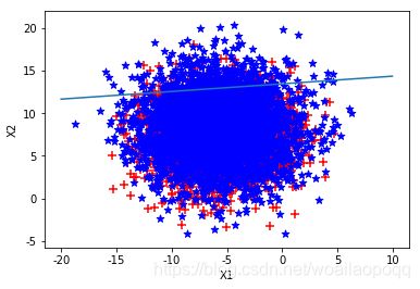
    x = np.arange(-20, 10, 0.05)
    y = -(weights[0, 0] +weights[1, 0] * x) / weights[2, 0]  #matix
    ax.plot(x, y)
    plt.xlabel('X1')
    plt.ylabel('X2')
    plt.savefig('image.png')
    plt.show()
   
    return weights


def init_data(data_file_name,init_random_state,length):
    #生成二分类数据，根据参数不同，生成的数据分类也不同，可以观察实际效果，最终ROC、KS都有变化
    randam_data, randam_target = make_blobs(n_features=2, n_samples=length, centers=2, random_state=init_random_state, cluster_std=[3,3.5])
    df = pd.DataFrame(randam_data,randam_target)
    df['target'] = randam_target
    df['x0']=1
    df.columns = ['x1','x2','y','x0']
    df.to_csv(data_file_name,index=False)
    
    df1 = df[df['y']==0]
    df2 = df[df['y']==1]
    df1.index = range(len(df1))
    df2.index = range(len(df2))
    
    fig = plt.figure()
    ax = fig.add_subplot(111)
    ax.scatter(df1['x1'],df1['x2'],marker='+',label='1',s=50,c='r')
    ax.scatter(df2['x1'],df2['x2'],marker='*',label='1',s=50,c='b')
    plt.xlabel('X1')
    plt.ylabel('X2')
    plt.savefig('image.png')
    plt.show()
def run(index):
    data_file_name = 'logistic_regression_data'
    file_name = data_file_name+'_'+str(index)+'.csv'
    init_data(file_name,index+1,10000)

    data = pd.read_csv(file_name)
    Xtrain, Xtest, Ytrain, Ytest = train_test_split(data,data['y'],test_size=0.3)
    weights = grad_descent(Xtrain,0.01,10000)
    
    #测试集进行验证
    w=weights[0, 0]*Xtest['x0']+weights[1, 0]*Xtest['x1']+weights[2, 0]*Xtest['x2']
    sm_y_probability = sigmoid(w)
    
    
    sm_y_pred = np.where(sm_y_probability >= 0.5,1,0)
#    cm = confusion_matrix(Xtest['y'],sm_y_pred,label=[0,1])
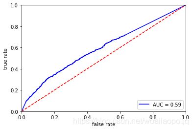
    fpr,tpr,threshold = metrics.roc_curve(Ytest,sm_y_probability)
    
    
    #计算ROC，并绘制曲线
    rocauc = auc(fpr, tpr)
    plt.plot(fpr, tpr, 'b', label='AUC = %0.2f' % rocauc)
    plt.legend(loc='lower right')
    plt.plot([0, 1], [0, 1], 'r--')
    plt.xlim([0, 1])
    plt.ylim([0, 1])
    plt.ylabel('true rate')
    plt.xlabel('false rate')
    plt.show()
        
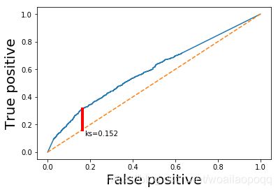
    ks_value = max(abs(fpr-tpr))
    #ROC曲线
    plt.plot(fpr, tpr)
    plt.plot([0,1], [0,1], linestyle='--')
    #绘制KS
    x = np.argwhere(abs(fpr-tpr) == ks_value)[0, 0]
    plt.plot([fpr[x], fpr[x]], [fpr[x], tpr[x]], linewidth=4, color='r')
    plt.text(fpr[x]+0.01,tpr[x]-0.2, 'ks='+str(format(ks_value,'0.3f')),color= 'black')
    plt.xlabel('False positive', fontsize=20)
    plt.ylabel('True positive', fontsize=20)
    plt.show()
def main():
    #数据格式 x0|x1|x2|y,其中x0列为1，程序自动生成训练的数据
    run(2)
    run(3)
    run(4)
    run(5)
    run(6)
if __name__ == '__main__':
    main()