g2o--icp代码解析

概要

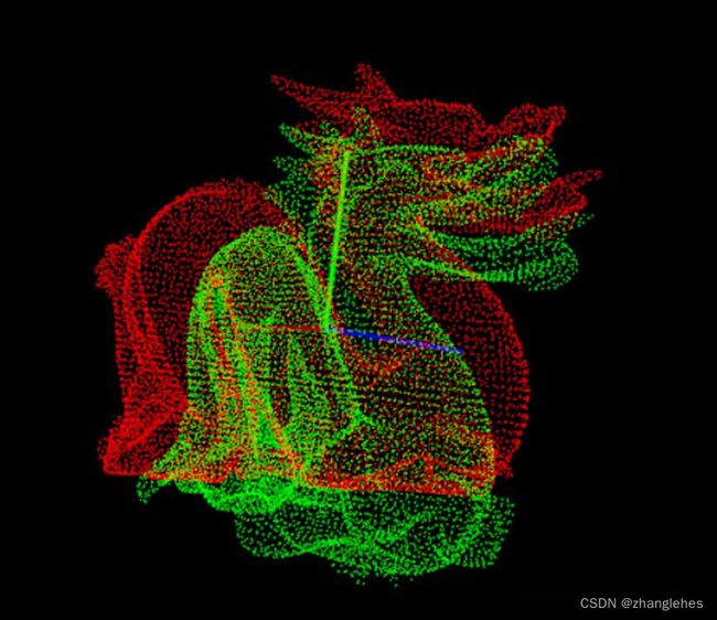
个人理解Icp是一种location算法。我们先将全局的事物特征化，提取出特征点。在求解过程中，将观察的的图像，同样进行特征化。将全局点与当前特征点进行匹配，就可以求得观察者当前的位姿。

Icp算法通常分为粗匹配和精细匹配两部分。粗匹配是将观察特征点移动到对应全局特征点的附近，而精细匹配这是将一个一个对应的特征点，使用最小二乘优化进行调整。在精细匹配的过程中，特征点对的选取也很重要，icp是一套迭代的算法，每次变换后都需要重新选取特征点对。

在求解一次特征点对匹配过程中，也存在很多中算法。笔者接触过的牛顿法思路比较简单，效果也很好。网上还推荐一种常用的方法svd，也是基于矩阵进行运算。今天介绍的g2o也是一种icp的匹配算法。

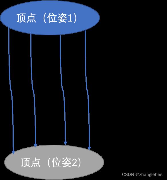
所谓的图优化，就是把一个常规的优化问题，以图（Graph）的形式来表述。在图中，以顶点表示优化变量，以边表示观测方程。于是总体优化问题变为n条边加和的形式(边是约束)。

所谓的问题

观测者所在两个位姿，能够看到特征点在自我坐标下的三维位置，并且在两个位姿下的特征点对是明确的，求解两个位姿的相对关系。

建图

源码解析

本文分析的也是g2o自带example中的代码（gicp_demo.cpp）

初始化求解器

  SparseOptimizer optimizer;
  optimizer.setVerbose(false);

  // variable-size block solver
  g2o::OptimizationAlgorithmLevenberg* solver =
      new g2o::OptimizationAlgorithmLevenberg(std::make_unique(
          std::make_unique<
              LinearSolverDense>()));

  optimizer.setAlgorithm(solver);

初始化1000个特征点

  vector true_points;
  for (size_t i = 0; i < 1000; ++i) {
    true_points.push_back(
        Vector3d((g2o::Sampler::uniformRand(0., 1.) - 0.5) * 3,
                 g2o::Sampler::uniformRand(0., 1.) - 0.5,
                 g2o::Sampler::uniformRand(0., 1.) + 10));
  }

初始化观测者的两个位姿

  // set up two poses
  int vertex_id = 0;
  for (size_t i = 0; i < 2; ++i) {
    // set up rotation and translation for this node
    Vector3d t(0, 0, i);
    Quaterniond q;
    q.setIdentity();

    Eigen::Isometry3d cam;  // camera pose
    cam = q;
    cam.translation() = t;

    // set up node
    VertexSE3* vc = new VertexSE3();
    vc->setEstimate(cam); // 设定初始位姿

    vc->setId(vertex_id);  // vertex id

    cerr << t.transpose() << " | " << q.coeffs().transpose() << endl;

    // set first cam pose fixed
    if (i == 0) vc->setFixed(true); // 将第一个点固定

    // add to optimizer
    optimizer.addVertex(vc); // 将观测者的位姿添加进优化器中

    vertex_id++;
  } 

添加约束

  // set up point matches
  for (size_t i = 0; i < true_points.size(); ++i) { // 遍历所有特征点
    // get two poses
    VertexSE3* vp0 =
        dynamic_cast(optimizer.vertices().find(0)->second); // 取出观测者第一个位姿
    VertexSE3* vp1 =
        dynamic_cast(optimizer.vertices().find(1)->second); // 取出观测者第二个位姿

    // calculate the relative 3D position of the point
    Vector3d pt0, pt1;
    pt0 = vp0->estimate().inverse() * true_points[i]; // 计算特征点在第一个位姿坐标系下的位置
    pt1 = vp1->estimate().inverse() * true_points[i]; // 计算特征点在第二个位姿坐标系下的位置

    // add in noise
    pt0 += Vector3d(g2o::Sampler::gaussRand(0., euc_noise), // 添加误差
                    g2o::Sampler::gaussRand(0., euc_noise),
                    g2o::Sampler::gaussRand(0., euc_noise));

    pt1 += Vector3d(g2o::Sampler::gaussRand(0., euc_noise),
                    g2o::Sampler::gaussRand(0., euc_noise),
                    g2o::Sampler::gaussRand(0., euc_noise));


    // form edge, with normals in varioius positions
    Vector3d nm0, nm1;
    nm0 << 0, i, 1;
    nm1 << 0, i, 1;
    nm0.normalize();
    nm1.normalize();

    Edge_V_V_GICP* e  // new edge with correct cohort for caching
        = new Edge_V_V_GICP();

    e->setVertex(0, vp0);  // first viewpoint 设定边的第一个顶点                                                 
    e->setVertex(1, vp1);  // second viewpoint 设定边的第二个顶点   

    EdgeGICP meas;
    meas.pos0 = pt0; // 设定边中第一个观测点的观测值
    meas.pos1 = pt1; // 设定边中第二个观测点的观测值
    meas.normal0 = nm0;
    meas.normal1 = nm1;

    e->setMeasurement(meas); // 设定观测值
    //        e->inverseMeasurement().pos() = -kp;

    meas = e->measurement();
    // use this for point-plane
    e->information() = meas.prec0(0.01); // 设定权重
    optimizer.addEdge(e); // 将该边添加进求解器中
  }

求解结果

  cout << endl << "Second vertex should be near 0,0,1" << endl;
  cout << dynamic_cast(optimizer.vertices().find(0)->second)
              ->estimate()
              .translation()
              .transpose()
       << endl;
  cout << dynamic_cast(optimizer.vertices().find(1)->second) // 第二个点的位姿是我们最关心的
              ->estimate()
              .translation()
              .transpose()
       << endl;

注：

关于边中的normal0和normal1参数的解释 -- https://github.com/RainerKuemmerle/g2o/issues/266