Keras深度学习框架实战(2):估计模型训练所需的样本量
1、模型训练样本量评估概述
1.1 样本量评估的意义
预估模型需要的样本量对于机器学习项目的成功至关重要,以下是几个主要原因:
-
防止过拟合与欠拟合:
- 过拟合:当模型在训练数据上表现极好,但在未见过的测试数据上表现糟糕时,就发生了过拟合。这通常是因为模型过于复杂,而训练数据不足以支持其学习数据的真实模式。通过预估足够的样本量,我们可以减少过拟合的风险。
- 欠拟合:与过拟合相反,欠拟合是模型未能捕捉到数据中的关键模式。这可能是因为模型过于简单或训练数据不足。预估样本量有助于确保模型有足够的数据来学习数据的复杂模式。
-
资源分配:
- 预估样本量有助于项目团队合理分配资源。如果预计需要大量数据,团队可以提前开始数据收集工作,或考虑使用更高效的数据收集方法。此外,了解所需样本量还可以帮助团队估算项目的时间和成本。
-
实验设计:
- 在设计实验或研究时,预估样本量有助于确定实验的规模。这有助于确保实验具有足够的统计功效,以检测感兴趣的效应或差异。
-
模型性能评估:
- 有了足够的样本量,我们可以更准确地评估模型的性能。通过将模型应用于独立的测试集,我们可以评估模型在未见过的数据上的表现,并据此调整模型参数或结构。
-
可解释性与泛化能力:
- 充足的样本量有助于模型学习数据的普遍规律,而不仅仅是训练数据的特定模式。这使得模型更有可能在类似但不同的数据集上表现良好,即具有更强的泛化能力。此外,充足的样本量还可以提高模型的可解释性,使结果更易于理解和解释给非技术利益相关者。
-
合规性与伦理:
- 在某些领域,如医疗、金融和法律等,数据收集和使用受到严格的法规和伦理准则的约束。预估样本量有助于确保项目符合这些要求,避免潜在的合规性问题和伦理争议。
-
提高项目成功率:
- 通过预估模型需要的样本量,项目团队可以更好地规划和管理项目资源。这有助于提高项目的成功率和效率,减少因资源不足或分配不当而导致的延误和失败。
预估模型需要的样本量是机器学习项目成功的关键一步。通过仔细考虑和计算所需的样本量,我们可以确保模型具有足够的数据来学习数据的真实模式,并减少过拟合和欠拟合的风险。同时,这还有助于项目团队更好地规划和管理资源,提高项目的成功率和效率。
1.2 样本量评估的一般方法
在许多现实世界的场景中,用于训练深度学习模型的图像数据量是有限的。特别是在医疗成像领域,数据集的创建成本高昂。当面临一个新的问题时,通常首先出现的问题是:“我们需要多少张图像来训练一个足够好的机器学习模型?”
在大多数情况下,只有一小部分样本可用,我们可以利用这些样本来模拟训练数据大小与模型性能之间的关系。这样的模型可以用于估计达到所需模型性能所需的最优图像数量。
样本量确定方法
-
平衡子采样方案:
- 在这个例子中,使用平衡子采样方案来确定模型的最佳样本量。该方案通过选择由Y个图像组成的随机子样本,并使用该子样本训练模型来完成。
- 随后,在一个独立的测试集上对模型进行评估。
- 该过程对每个子样本重复N次,并进行替换,以构建观测性能的平均值和置信区间。
-
样本量与模型性能的关系建模:
- 利用现有的一小部分样本,我们可以构建一个模型来模拟训练数据大小与模型性能之间的关系。
- 这个模型可以帮助我们预测,随着训练数据量的增加,模型性能将如何变化。
-
最优样本量的估计:
- 通过分析模型性能与训练数据大小之间的关系,我们可以估计出达到特定性能水平所需的最优样本量。
- 这有助于我们确定在资源限制下,应收集多少图像来训练模型。
-
重复实验与统计评估:
- 为了获得更准确的估计,我们重复上述过程多次,并计算观测性能的平均值和置信区间。
- 这有助于我们评估估计的可靠性,并确定所需的样本量是否足够稳健。
通过采用平衡子采样方案和构建模型性能与训练数据大小之间的关系模型,我们可以系统地估计出达到所需模型性能所需的最优图像数量。这种方法不仅可以帮助我们在有限的资源下做出明智的决策,还可以提高机器学习模型在实际应用中的性能和可靠性。在医疗成像等数据稀缺的领域,这种方法尤为重要。
2、设置
import os

os.environ["KERAS_BACKEND"] = "tensorflow"

import matplotlib.pyplot as plt
import numpy as np
import tensorflow as tf
import keras
from keras import layers
import tensorflow_datasets as tfds

# Define seed and fixed variables
seed = 42
keras.utils.set_random_seed(seed)
AUTO = tf.data.AUTOTUNE
3、数据集加载
我们将使用 TF Flowers 数据集,加载它并将其转换为 NumPy 数组。
数据下载地址如下:
https://storage.googleapis.com/download.tensorflow.org/example_images/flower_photos.tgz
下面是一个示例代码,展示如何使用 TensorFlow 的 tf.keras.preprocessing.image_dataset_from_directory 函数加载数据集,并将其转换为 NumPy 数组:
# Specify dataset parameters
dataset_name = "tf_flowers"
batch_size = 64
image_size = (224, 224)

# Load data from tfds and split 10% off for a test set
(train_data, test_data), ds_info = tfds.load(
    dataset_name,
    split=["train[:90%]", "train[90%:]"],
    shuffle_files=True,
    as_supervised=True,
    with_info=True,
)

# Extract number of classes and list of class names
num_classes = ds_info.features["label"].num_classes
class_names = ds_info.features["label"].names

print(f"Number of classes: {num_classes}")
print(f"Class names: {class_names}")


# Convert datasets to NumPy arrays
def dataset_to_array(dataset, image_size, num_classes):
    images, labels = [], []
    for img, lab in dataset.as_numpy_iterator():
        images.append(tf.image.resize(img, image_size).numpy())
        labels.append(tf.one_hot(lab, num_classes))
    return np.array(images), np.array(labels)


img_train, label_train = dataset_to_array(train_data, image_size, num_classes)
img_test, label_test = dataset_to_array(test_data, image_size, num_classes)

num_train_samples = len(img_train)
print(f"Number of training samples: {num_train_samples}")
Number of classes: 5
Class names: ['dandelion', 'daisy', 'tulips', 'sunflowers', 'roses']
Number of training samples: 3303
从测试集中绘制几个示例的图表
plt.figure(figsize=(16, 12))
for n in range(30):
    ax = plt.subplot(5, 6, n + 1)
    plt.imshow(img_test[n].astype("uint8"))
    plt.title(np.array(class_names)[label_test[n] == True][0])
    plt.axis("off")
4、图像增强(Augmentation)
使用Keras预处理层(preprocessing layers)定义图像增强,并将其应用于训练集。
在深度学习中,图像增强是一种常用的技术,用于通过随机修改训练图像来增加模型的泛化能力。这些修改可能包括旋转、缩放、翻转、裁剪、颜色变换等。通过使用Keras的预处理层,您可以轻松地为训练数据定义和执行这些增强操作。
# Define image augmentation model
image_augmentation = keras.Sequential(
    [
        layers.RandomFlip(mode="horizontal"),
        layers.RandomRotation(factor=0.1),
        layers.RandomZoom(height_factor=(-0.1, -0)),
        layers.RandomContrast(factor=0.1),
    ],
)

# Apply the augmentations to the training images and plot a few examples
img_train = image_augmentation(img_train).numpy()

plt.figure(figsize=(16, 12))
for n in range(30):
    ax = plt.subplot(5, 6, n + 1)
    plt.imshow(img_train[n].astype("uint8"))
    plt.title(np.array(class_names)[label_train[n] == True][0])
    plt.axis("off")
5、定义模型构建和训练函数
我们创建几个方便的函数来构建基于迁移学习的模型,编译并训练它,以及解冻层以进行微调。
def train_model(training_data, training_labels):
    """Trains the model as follows:

    - Trains only the top layers for 10 epochs.
    - Unfreezes deeper layers.
    - Train for 20 more epochs.

    Arguments:
        training_data: NumPy Array, training data.
        training_labels: NumPy Array, training labels.

    Returns:
        Model accuracy.
    """

    model = build_model(num_classes)

    # Compile and train top layers
    history = compile_and_train(
        model,
        training_data,
        training_labels,
        metrics=[keras.metrics.AUC(name="auc"), "acc"],
        optimizer=keras.optimizers.Adam(),
        patience=3,
        epochs=10,
    )

    # Unfreeze model from block 10 onwards
    model = unfreeze(model, "block_10")

    # Compile and train for 20 epochs with a lower learning rate
    fine_tune_epochs = 20
    total_epochs = history.epoch[-1] + fine_tune_epochs

    history_fine = compile_and_train(
        model,
        training_data,
        training_labels,
        metrics=[keras.metrics.AUC(name="auc"), "acc"],
        optimizer=keras.optimizers.Adam(learning_rate=1e-4),
        patience=5,
        epochs=total_epochs,
    )

    # Calculate model accuracy on the test set
    _, _, acc = model.evaluate(img_test, label_test)
    return np.round(acc, 4)
6、迭代训练模型
既然我们已经有了模型构建函数和支持迭代训练的函数,我们就可以在几个子样本分割上迭代训练模型。
我们选择子样本分割为下载数据集的5%、10%、25%和50%。我们假设目前只有50%的实际数据是可用的。
我们在每个分割上从零开始训练模型5次,并记录准确率值。
请注意,这将训练20个模型,并需要一些时间。请确保您已经激活了GPU运行环境。
为了保持这个示例的轻量级,我们提供了之前训练运行的样本数据。
def train_iteratively(sample_splits=[0.05, 0.1, 0.25, 0.5], iter_per_split=5):
    """Trains a model iteratively over several sample splits.

    Arguments:
        sample_splits: List/NumPy array, contains fractions of the trainins set
                        to train over.
        iter_per_split: Int, number of times to train a model per sample split.

    Returns:
        Training accuracy for all splits and iterations and the number of samples
        used for training at each split.
    """
    # Train all the sample models and calculate accuracy
    train_acc = []
    sample_sizes = []

    for fraction in sample_splits:
        print(f"Fraction split: {fraction}")
        # Repeat training 3 times for each sample size
        sample_accuracy = []
        num_samples = int(num_train_samples * fraction)
        for i in range(iter_per_split):
            print(f"Run {i+1} out of {iter_per_split}:")
            # Create fractional subsets
            rand_idx = np.random.randint(num_train_samples, size=num_samples)
            train_img_subset = img_train[rand_idx, :]
            train_label_subset = label_train[rand_idx, :]
            # Train model and calculate accuracy
            accuracy = train_model(train_img_subset, train_label_subset)
            print(f"Accuracy: {accuracy}")
            sample_accuracy.append(accuracy)
        train_acc.append(sample_accuracy)
        sample_sizes.append(num_samples)
    return train_acc, sample_sizes


# Running the above function produces the following outputs
train_acc = [
    [0.8202, 0.7466, 0.8011, 0.8447, 0.8229],
    [0.861, 0.8774, 0.8501, 0.8937, 0.891],
    [0.891, 0.9237, 0.8856, 0.9101, 0.891],
    [0.8937, 0.9373, 0.9128, 0.8719, 0.9128],
]

sample_sizes = [165, 330, 825, 1651]
7、学习曲线
我们现在通过拟合一个指数曲线穿过平均准确率点来绘制学习曲线。我们使用TensorFlow(TF)来通过数据拟合一个指数函数。
然后,我们扩展学习曲线来预测在整个训练集上训练的模型的准确率。
绘制学习曲线通常用于理解模型在拥有不同数量的训练数据时的性能如何变化。通过观察随着数据量增加时模型准确率的提升(或停滞),我们可以对模型的学习能力有一个大致的了解,并可能发现是否存在过拟合或欠拟合的问题。
在训练数据有限的情况下,通过外推学习曲线,我们可以对使用更多数据(例如整个训练集)时模型的潜在性能进行预测。这有助于我们决定是否值得进一步收集或生成更多的训练数据。
def fit_and_predict(train_acc, sample_sizes, pred_sample_size):
    """Fits a learning curve to model training accuracy results.

    Arguments:
        train_acc: List/Numpy Array, training accuracy for all model
                    training splits and iterations.
        sample_sizes: List/Numpy array, number of samples used for training at
                    each split.
        pred_sample_size: Int, sample size to predict model accuracy based on
                        fitted learning curve.
    """
    x = sample_sizes
    mean_acc = tf.convert_to_tensor([np.mean(i) for i in train_acc])
    error = [np.std(i) for i in train_acc]

    # Define mean squared error cost and exponential curve fit functions
    mse = keras.losses.MeanSquaredError()

    def exp_func(x, a, b):
        return a * x**b

    # Define variables, learning rate and number of epochs for fitting with TF
    a = tf.Variable(0.0)
    b = tf.Variable(0.0)
    learning_rate = 0.01
    training_epochs = 5000

    # Fit the exponential function to the data
    for epoch in range(training_epochs):
        with tf.GradientTape() as tape:
            y_pred = exp_func(x, a, b)
            cost_function = mse(y_pred, mean_acc)
        # Get gradients and compute adjusted weights
        gradients = tape.gradient(cost_function, [a, b])
        a.assign_sub(gradients[0] * learning_rate)
        b.assign_sub(gradients[1] * learning_rate)
    print(f"Curve fit weights: a = {a.numpy()} and b = {b.numpy()}.")

    # We can now estimate the accuracy for pred_sample_size
    max_acc = exp_func(pred_sample_size, a, b).numpy()

    # Print predicted x value and append to plot values
    print(f"A model accuracy of {max_acc} is predicted for {pred_sample_size} samples.")
    x_cont = np.linspace(x[0], pred_sample_size, 100)

    # Build the plot
    fig, ax = plt.subplots(figsize=(12, 6))
    ax.errorbar(x, mean_acc, yerr=error, fmt="o", label="Mean acc & std dev.")
    ax.plot(x_cont, exp_func(x_cont, a, b), "r-", label="Fitted exponential curve.")
    ax.set_ylabel("Model classification accuracy.", fontsize=12)
    ax.set_xlabel("Training sample size.", fontsize=12)
    ax.set_xticks(np.append(x, pred_sample_size))
    ax.set_yticks(np.append(mean_acc, max_acc))
    ax.set_xticklabels(list(np.append(x, pred_sample_size)), rotation=90, fontsize=10)
    ax.yaxis.set_tick_params(labelsize=10)
    ax.set_title("Learning curve: model accuracy vs sample size.", fontsize=14)
    ax.legend(loc=(0.75, 0.75), fontsize=10)
    ax.xaxis.grid(True)
    ax.yaxis.grid(True)
    plt.tight_layout()
    plt.show()

    # The mean absolute error (MAE) is calculated for curve fit to see how well
    # it fits the data. The lower the error the better the fit.
    mae = keras.losses.MeanAbsoluteError()
    print(f"The mae for the curve fit is {mae(mean_acc, exp_func(x, a, b)).numpy()}.")


# We use the whole training set to predict the model accuracy
fit_and_predict(train_acc, sample_sizes, pred_sample_size=num_train_samples)
Curve fit weights: a = 0.6445642113685608 and b = 0.048097413033246994.
A model accuracy of 0.9517362117767334 is predicted for 3303 samples.
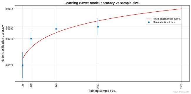
从外推曲线中我们可以看到,使用3303张图像将产生大约95%的估计准确率。
让我们使用所有数据(3303张图像)来训练模型,看看我们的预测是否准确!
# Now train the model with full dataset to get the actual accuracy
accuracy = train_model(img_train, label_train)
print(f"A model accuracy of {accuracy} is reached on {num_train_samples} images!")
Trainable weights: 2
Non_trainable weights: 260
Epoch 1/10
 47/47 ━━━━━━━━━━━━━━━━━━━━ 18s 338ms/step - acc: 0.4305 - auc: 0.7221 - loss: 1.4585 - val_acc: 0.8218 - val_auc: 0.9700 - val_loss: 0.5043
Epoch 2/10
 47/47 ━━━━━━━━━━━━━━━━━━━━ 15s 326ms/step - acc: 0.7666 - auc: 0.9504 - loss: 0.6287 - val_acc: 0.8792 - val_auc: 0.9838 - val_loss: 0.3733
Epoch 3/10
 47/47 ━━━━━━━━━━━━━━━━━━━━ 16s 332ms/step - acc: 0.8252 - auc: 0.9673 - loss: 0.5039 - val_acc: 0.8852 - val_auc: 0.9880 - val_loss: 0.3182
Epoch 4/10
 47/47 ━━━━━━━━━━━━━━━━━━━━ 16s 348ms/step - acc: 0.8458 - auc: 0.9768 - loss: 0.4264 - val_acc: 0.8822 - val_auc: 0.9893 - val_loss: 0.2956
Epoch 5/10
 47/47 ━━━━━━━━━━━━━━━━━━━━ 16s 350ms/step - acc: 0.8661 - auc: 0.9812 - loss: 0.3821 - val_acc: 0.8912 - val_auc: 0.9903 - val_loss: 0.2755
Epoch 6/10
 47/47 ━━━━━━━━━━━━━━━━━━━━ 16s 336ms/step - acc: 0.8656 - auc: 0.9836 - loss: 0.3555 - val_acc: 0.9003 - val_auc: 0.9906 - val_loss: 0.2701
Epoch 7/10
 47/47 ━━━━━━━━━━━━━━━━━━━━ 16s 331ms/step - acc: 0.8800 - auc: 0.9846 - loss: 0.3430 - val_acc: 0.8943 - val_auc: 0.9914 - val_loss: 0.2548
Epoch 8/10
 47/47 ━━━━━━━━━━━━━━━━━━━━ 16s 333ms/step - acc: 0.8917 - auc: 0.9871 - loss: 0.3143 - val_acc: 0.8973 - val_auc: 0.9917 - val_loss: 0.2494
Epoch 9/10
 47/47 ━━━━━━━━━━━━━━━━━━━━ 15s 320ms/step - acc: 0.9003 - auc: 0.9891 - loss: 0.2906 - val_acc: 0.9063 - val_auc: 0.9908 - val_loss: 0.2463
Epoch 10/10
 47/47 ━━━━━━━━━━━━━━━━━━━━ 15s 324ms/step - acc: 0.8997 - auc: 0.9895 - loss: 0.2839 - val_acc: 0.9124 - val_auc: 0.9912 - val_loss: 0.2394
Trainable weights: 24
Non-trainable weights: 238
Epoch 1/29
 47/47 ━━━━━━━━━━━━━━━━━━━━ 27s 537ms/step - acc: 0.8457 - auc: 0.9747 - loss: 0.4365 - val_acc: 0.9094 - val_auc: 0.9916 - val_loss: 0.2692
Epoch 2/29
 47/47 ━━━━━━━━━━━━━━━━━━━━ 24s 502ms/step - acc: 0.9223 - auc: 0.9932 - loss: 0.2198 - val_acc: 0.9033 - val_auc: 0.9891 - val_loss: 0.2826
Epoch 3/29
 47/47 ━━━━━━━━━━━━━━━━━━━━ 25s 534ms/step - acc: 0.9499 - auc: 0.9972 - loss: 0.1399 - val_acc: 0.9003 - val_auc: 0.9910 - val_loss: 0.2804
Epoch 4/29
 47/47 ━━━━━━━━━━━━━━━━━━━━ 26s 554ms/step - acc: 0.9590 - auc: 0.9983 - loss: 0.1130 - val_acc: 0.9396 - val_auc: 0.9968 - val_loss: 0.1510
Epoch 5/29
 47/47 ━━━━━━━━━━━━━━━━━━━━ 25s 533ms/step - acc: 0.9805 - auc: 0.9996 - loss: 0.0538 - val_acc: 0.9486 - val_auc: 0.9914 - val_loss: 0.1795
Epoch 6/29
 47/47 ━━━━━━━━━━━━━━━━━━━━ 24s 516ms/step - acc: 0.9949 - auc: 1.0000 - loss: 0.0226 - val_acc: 0.9124 - val_auc: 0.9833 - val_loss: 0.3186
Epoch 7/29
 47/47 ━━━━━━━━━━━━━━━━━━━━ 25s 534ms/step - acc: 0.9900 - auc: 0.9999 - loss: 0.0297 - val_acc: 0.9275 - val_auc: 0.9881 - val_loss: 0.3017
Epoch 8/29
 47/47 ━━━━━━━━━━━━━━━━━━━━ 25s 536ms/step - acc: 0.9910 - auc: 0.9999 - loss: 0.0228 - val_acc: 0.9426 - val_auc: 0.9927 - val_loss: 0.1938
Epoch 9/29
 47/47 ━━━━━━━━━━━━━━━━━━━━ 0s 489ms/step - acc: 0.9995 - auc: 1.0000 - loss: 0.0069Restoring model weights from the end of the best epoch: 4.
 47/47 ━━━━━━━━━━━━━━━━━━━━ 25s 527ms/step - acc: 0.9995 - auc: 1.0000 - loss: 0.0068 - val_acc: 0.9426 - val_auc: 0.9919 - val_loss: 0.2957
Epoch 9: early stopping
 12/12 ━━━━━━━━━━━━━━━━━━━━ 2s 170ms/step - acc: 0.9641 - auc: 0.9972 - loss: 0.1264
A model accuracy of 0.9964 is reached on 3303 images!
8、结论
我们看到,使用3303张图像,模型达到了约94-96%的准确率。这与我们的估计非常接近!
尽管我们只使用了数据集的50%(1651张图像),但我们能够模拟模型的训练行为,并预测给定图像数量下的模型准确率。同样的方法可以用于预测达到所需准确率所需的图像数量。这在数据量较小时非常有用,当已经显示出深度学习模型可以收敛,但需要更多图像时。图像数量的预测可以用于计划和预算进一步的图像收集工作。