《Python实战进阶》No34：卷积神经网络（CNN）图像分类实战

第34集：卷积神经网络（CNN）图像分类实战

---

摘要

卷积神经网络（CNN）是计算机视觉领域的核心技术，特别擅长处理图像分类任务。本集将深入讲解 CNN 的核心组件（卷积层、池化层、全连接层），并演示如何使用 PyTorch 构建一个完整的 CNN 模型，在 CIFAR-10 数据集上实现图像分类。我们还将探讨数据增强和正则化技术（如 Dropout 和 BatchNorm）对模型性能的影响。

---

核心概念和知识点

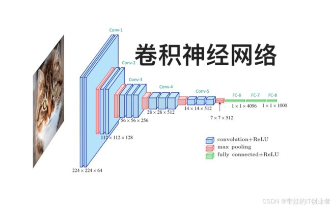
1. CNN 的核心组件

• 卷积层：通过滤波器（Filter）提取局部特征（如边缘、纹理）。
• 池化层：通过下采样（如最大池化）减少参数数量，增强特征鲁棒性。
• 全连接层：将提取的特征映射到分类标签。

2. 数据增强技术

• 常用方法：随机水平翻转、随机裁剪、色彩抖动（调整亮度、对比度）。
• 作用：增加训练数据的多样性，防止过拟合。

3. 过拟合与正则化

• 过拟合：模型在训练集表现优异，但在测试集性能下降。
• 正则化方法：
  • Dropout：随机关闭部分神经元，减少对特定特征的依赖。
  • BatchNorm：标准化每层的输入，加速训练并提升泛化能力。

4. 与 AI 大模型的关联

• 基础架构角色：CNN 是许多大模型（如 ResNet、EfficientNet）的核心组件。
• 迁移学习：通过预训练的 CNN 模型（如 ImageNet 权重）快速适应新任务。
• 自监督学习：利用 CNN 提取特征，用于无标签数据的预训练。

---

实战案例：使用 CNN 分类 CIFAR-10 数据集

背景

CIFAR-10 包含 60,000 张 32x32 彩色图像，分为 10 个类别（飞机、汽车、鸟类等）。我们将构建一个轻量级 CNN 模型，结合数据增强和正则化技术提升分类性能。

代码实现

1. 环境准备

import torch
import torch.nn as nn
import torch.optim as optim
import torchvision
import torchvision.transforms as transforms
import matplotlib.pyplot as plt
import numpy as np
from torch.utils.data import DataLoader

2. 数据加载和预处理

def load_data():
    # 数据增强
    transform_train = transforms.Compose([
        transforms.RandomCrop(32, padding=4),
        transforms.RandomHorizontalFlip(),
        transforms.RandomRotation(15),
        transforms.ToTensor(),
        transforms.Normalize((0.4914, 0.4822, 0.4465), 
                           (0.2023, 0.1994, 0.2010))
    ])
    
    transform_test = transforms.Compose([
        transforms.ToTensor(),
        transforms.Normalize((0.4914, 0.4822, 0.4465), 
                           (0.2023, 0.1994, 0.2010))
    ])
    
    # 加载CIFAR-10数据集
    trainset = torchvision.datasets.CIFAR10(
        root='./data', train=True, download=True, transform=transform_train)
    testset = torchvision.datasets.CIFAR10(
        root='./data', train=False, download=True, transform=transform_test)
    
    return trainset, testset

3. 构建CNN模型

class CNN(nn.Module):
    def __init__(self):
        super(CNN, self).__init__()
        
        # 第一个卷积块
        self.conv1 = nn.Conv2d(3, 32, kernel_size=3, padding=1)
        self.bn1 = nn.BatchNorm2d(32)
        self.conv2 = nn.Conv2d(32, 32, kernel_size=3, padding=1)
        self.bn2 = nn.BatchNorm2d(32)
        self.pool1 = nn.MaxPool2d(kernel_size=2, stride=2)
        self.dropout1 = nn.Dropout(0.25)
        
        # 第二个卷积块
        self.conv3 = nn.Conv2d(32, 64, kernel_size=3, padding=1)
        self.bn3 = nn.BatchNorm2d(64)
        self.conv4 = nn.Conv2d(64, 64, kernel_size=3, padding=1)
        self.bn4 = nn.BatchNorm2d(64)
        self.pool2 = nn.MaxPool2d(kernel_size=2, stride=2)
        self.dropout2 = nn.Dropout(0.25)
        
        # 第三个卷积块
        self.conv5 = nn.Conv2d(64, 128, kernel_size=3, padding=1)
        self.bn5 = nn.BatchNorm2d(128)
        self.conv6 = nn.Conv2d(128, 128, kernel_size=3, padding=1)
        self.bn6 = nn.BatchNorm2d(128)
        self.pool3 = nn.MaxPool2d(kernel_size=2, stride=2)
        self.dropout3 = nn.Dropout(0.25)
        
        # 全连接层
        self.fc1 = nn.Linear(128 * 4 * 4, 512)
        self.dropout4 = nn.Dropout(0.5)
        self.fc2 = nn.Linear(512, 10)
        
    def forward(self, x):
        # 第一个卷积块
        x = self.pool1(F.relu(self.bn2(self.conv2(F.relu(self.bn1(self.conv1(x)))))))
        x = self.dropout1(x)
        
        # 第二个卷积块
        x = self.pool2(F.relu(self.bn4(self.conv4(F.relu(self.bn3(self.conv3(x)))))))
        x = self.dropout2(x)
        
        # 第三个卷积块
        x = self.pool3(F.relu(self.bn6(self.conv6(F.relu(self.bn5(self.conv5(x)))))))
        x = self.dropout3(x)
        
        # 全连接层
        x = x.view(-1, 128 * 4 * 4)
        x = self.dropout4(F.relu(self.fc1(x)))
        x = self.fc2(x)
        return x

4. 训练和评估

def train_model(model, trainloader, criterion, optimizer, device):
    model.train()
    running_loss = 0.0
    correct = 0
    total = 0
    
    for i, data in enumerate(trainloader):
        inputs, labels = data[0].to(device), data[1].to(device)
        
        optimizer.zero_grad()
        outputs = model(inputs)
        loss = criterion(outputs, labels)
        loss.backward()
        optimizer.step()
        
        running_loss += loss.item()
        _, predicted = outputs.max(1)
        total += labels.size(0)
        correct += predicted.eq(labels).sum().item()
        
        if (i + 1) % 100 == 0:
            print(f'Batch [{i + 1}], Loss: {running_loss/100:.4f}, '
                  f'Acc: {100.*correct/total:.2f}%')
            running_loss = 0.0

def evaluate_model(model, testloader, device):
    model.eval()
    correct = 0
    total = 0
    
    with torch.no_grad():
        for data in testloader:
            images, labels = data[0].to(device), data[1].to(device)
            outputs = model(images)
            _, predicted = outputs.max(1)
            total += labels.size(0)
            correct += predicted.eq(labels).sum().item()
    
    accuracy = 100. * correct / total
    print(f'测试集准确率: {accuracy:.2f}%')
    return accuracy

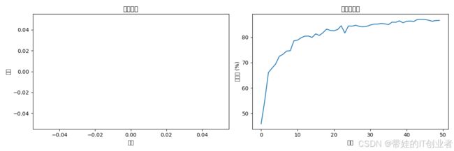
5. 可视化训练过程

def plot_training_history(train_losses, test_accuracies):
    plt.figure(figsize=(12, 4))
    
    # 绘制训练损失
    plt.subplot(1, 2, 1)
    plt.plot(train_losses)
    plt.title('训练损失')
    plt.xlabel('批次')
    plt.ylabel('损失')
    
    # 绘制测试准确率
    plt.subplot(1, 2, 2)
    plt.plot(test_accuracies)
    plt.title('测试准确率')
    plt.xlabel('轮次')
    plt.ylabel('准确率 (%)')
    
    plt.tight_layout()
    plt.show()

程序输出结果：

---

总结

通过本集的学习，我们掌握了 CNN 的核心组件和正则化技术，并通过 CIFAR-10 图像分类任务验证了模型的有效性。CNN 的卷积层和池化层能够有效提取图像特征，而数据增强与 Dropout/BatchNorm 的结合显著提升了模型的泛化能力。

---

扩展思考

1. 迁移学习提升模型性能

• 使用预训练模型（如 ResNet-18）作为特征提取器，仅微调最后几层。
• 代码示例：

  import torchvision.models as models
  resnet = models.resnet18(pretrained=True)
  # 冻结卷积层
  for param in resnet.parameters():
      param.requires_grad = False
  # 替换最后的全连接层
  resnet.fc = nn.Linear(resnet.fc.in_features, 10)
  

2. 自监督学习的潜力

• 自监督学习通过无标签数据预训练模型（如通过图像旋转预测任务），可在小数据集上取得更好的效果。
• 例如，使用 MoCo 框架预训练 CNN 编码器。

---

专栏链接：Python实战进阶
下期预告：No35：循环神经网络（RNN）时间序列预测