Auto-encoding Variational Bayes 阅读笔记

Notation

• pθ(z|x) p θ ( z | x ) : intractable posterior
• pθ(x|z) p θ ( x | z ) : probabilistic decoder
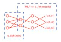
• qϕ(z|x) q ϕ ( z | x ) : recognition model, variational approximation to pθ(z|x) p θ ( z | x ) , also regarded as a probabilistic encoder
• pθ(z)pθ(x|z) p θ ( z ) p θ ( x | z ) : generative model
• ϕ ϕ : variational parameters
• θ θ : generative parameters

Abbreviation

• SGVB: Stochastic Gradient Variational Bayes
• AEVB: auto-encoding VB
• ML: maximum likelihood
• MAP: maximum a posteriori

---

Motivation

• Problem

  • How to perform efficient inference and learning in directed probabilistic models, in the presence of continuous latent variables with intractable posterior distribution pθ(z|x) p θ ( z | x ) and large datasets?

• Existing Solution and Difficulty

  • VB: involves the optimization of an approximation to the intractable posterior
  • mean-field: requires analytical solutions of expectations w.r.t. the approximate posterior, which are also intractable in the general case

---

Contribution of this paper

• (1) SGVB estimator: an estimator of the variational lower bound
  
  • yielded by a reparameterization of the variational lower bound
  • simple & differentiable & unbiased
  • straightforwad to optimize using standard SG ascent techniques
• (2) AEVB algorithm
  
  • using SGVB to optimize a recognition model that allows us to perform very efficient approximate posterior inference using simple ancestral sampling, which in turn allows us to efficiently learn the model parameters, without the need of expensive iterative inference schemes (such as MCMC) per datapoint.
  • condition: i.i.d. datasets X={x(i)}Ni=1 X = { x ( i ) } i = 1 N & continuous latent variable z z per datapoint

---

Methodology

assumption

• directed graphical models with continuous latent variables
• i.i.d. dataset with latent variables per datapoint
  
  • where we like to perform
    
    • ML or MAP inference on the (global) paramters θ θ
    • variational inference on the latent variable z z
• pθ(z) p θ ( z ) and pθ(x|z) p θ ( x | z ) : both PDFs are differentiable almost everywhere w.r.t. both θ θ and z z

target case

• intractability
  
  • pθ(x)=∫pθ(z)pθ(x|z)dz p θ ( x ) = ∫ p θ ( z ) p θ ( x | z ) d z : so we cannot evaluate or differentiate it.
  • pθ(z|x)=pθ(x|z)pθ(z)pθ(x) p θ ( z | x ) = p θ ( x | z ) p θ ( z ) p θ ( x ) : so the EM algorithm cannot be used.
  • the required integrals for any reasonable mean-field VB algorithm: so the VB algorithm cannot be used.
  • in cases of moderately complicated likelihood function, e.g. in a neural network with a nonlinear hidden layer
• a large dataset
  
  • batch optimization is too costly => minibatch or single datapoints
  • sampling bases solutions are too slow, e.g. Monte Carlo EM, since it involves a typically expensive sampling loop per datapoint.

solution and application

• efficient approximate ML or MAP estimation for θ θ (Full): Appendix F
  
  • allow us to mimic the hidden random process and generate artificial data that resemble the real data
• efficient approximate posterior inference pθ(z|x) p θ ( z | x ) for a choice of θ θ
  
  • useful for coding or data representation tasks
• efficient approximate marginal inference of x x : Appendix D
  
  • allow us to perform all kinds of inference tasks where p(x) p ( x ) is required, such as image denoising, inpainting, and super-resolution.

  1. derivation of the variational bound

  logpθ(x(1)，⋯,x(N))=∑i=1Nlogpθ(x(i)) log ⁡ p θ ( x ( 1 ) ， ⋯ , x ( N ) ) = ∑ i = 1 N log ⁡ p θ ( x ( i ) )
  
  Here we use xi x i to represent x(i) x ( i )
  logp(xi)=∫zq(z|xi)logp(xi)dz  (q can be any distribution)=∫zq(z|xi)logp(z,xi)p(z|xi)dz=∫zq(z|xi)log[q(z|xi)p(z|xi)⋅p(z,xi)q(z|xi)]dz=∫zq(z|xi)logq(z|xi)p(z|xi)dz+∫zq(z|xi)logp(z,xi)q(z|xi)dz=DKL[qϕ(z|xi)∥pθ(z|xi)]+LB(θ,ϕ;xi) log ⁡ p ( x i ) = ∫ z q ( z | x i ) log ⁡ p ( x i ) d z     ( q  can be any distribution) = ∫ z q ( z | x i ) log ⁡ p ( z , x i ) p ( z | x i ) d z = ∫ z q ( z | x i ) log ⁡ [ q ( z | x i ) p ( z | x i ) ⋅ p ( z , x i ) q ( z | x i ) ] d z = ∫ z q ( z | x i ) log ⁡ q ( z | x i ) p ( z | x i ) d z + ∫ z q ( z | x i ) log ⁡ p ( z , x i ) q ( z | x i ) d z = D K L [ q ϕ ( z | x i ) ∥ p θ ( z | x i ) ] + L B ( θ , ϕ ; x i )

  Becuase DKL≥0 D K L ≥ 0 , so LB L B is called the (variational) lower bound, then we have
  

  logpθ(xi)≥LB(θ,ϕ;xi) log ⁡ p θ ( x i ) ≥ L B ( θ , ϕ ; x i )
  LB(θ,ϕ;xi)=Eqϕ(z|x)[logpθ(x,z)−logqϕ(z|x)]=∫zq(z|xi)logp(z,xi)q(z|xi)dz=∫zq(z|xi)logp(xi|z)p(z)q(z|xi)dz=−DKL[q(z|xi)∥p(z)]+∫zq(z|xi)logp(xi|z)dz=−DKL[qϕ(z|xi)∥pθ(z)]+Eqϕ(z|xi)[logpθ(xi|z)] L B ( θ , ϕ ; x i ) = E q ϕ ( z | x ) [ log ⁡ p θ ( x , z ) − log ⁡ q ϕ ( z | x ) ] = ∫ z q ( z | x i ) log ⁡ p ( z , x i ) q ( z | x i ) d z = ∫ z q ( z | x i ) log ⁡ p ( x i | z ) p ( z ) q ( z | x i ) d z = − D K L [ q ( z | x i ) ∥ p ( z ) ] + ∫ z q ( z | x i ) log ⁡ p ( x i | z ) d z = − D K L [ q ϕ ( z | x i ) ∥ p θ ( z ) ] + E q ϕ ( z | x i ) [ log ⁡ p θ ( x i | z ) ]
  • −DKL[qϕ(z|xi)∥pθ(z)] − D K L [ q ϕ ( z | x i ) ∥ p θ ( z ) ] : act as a regularizer
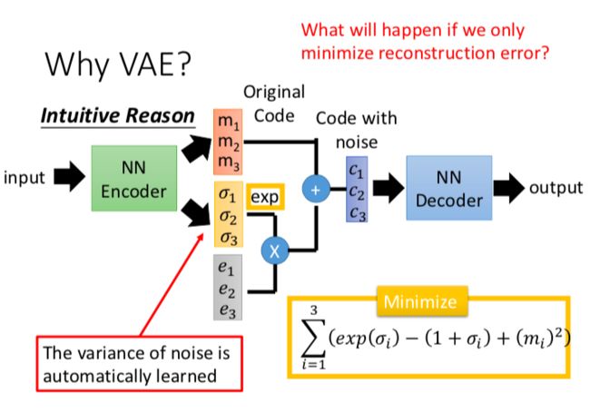
  • Eqϕ(z|xi)[logpθ(xi|z)] E q ϕ ( z | x i ) [ log ⁡ p θ ( x i | z ) ] : a an expected negative reconstruction error
  • TARGET: defferentiate and optimize LB L B w.r.t. both ϕ ϕ and θ θ . However, ∇ϕLB ∇ ϕ L B is problematic.

  2. Solution-1 Naive Monte Carlo gradient estimator

  • disadvantages: high variance & impractical for this purpose, 原文中出现的公式如下：
    
    ∇ϕEqϕ(z)[f(z)]=Eqϕ(z)[f(z)∇qϕ(z)logqϕ(z)]≃1L∑l=1Lf(z)∇qϕ(zl)logqϕ(zl)where zl∼qϕ(z|xi) ∇ ϕ E q ϕ ( z ) [ f ( z ) ] = E q ϕ ( z ) [ f ( z ) ∇ q ϕ ( z ) log ⁡ q ϕ ( z ) ] ≃ 1 L ∑ l = 1 L f ( z ) ∇ q ϕ ( z l ) log ⁡ q ϕ ( z l ) where   z l ∼ q ϕ ( z | x i )

  但由于我还没来得及学Monte Carlo Gradient Estimator的理论，根据VAE这边论文后面的公式，个人觉得…上面的公式应该是（数学功底不够深厚，不确定二者是否等价）：
  

  ∇ϕEqϕ(z)[f(z)]=Eqϕ(z)[f(z)∇qϕ(z)logqϕ(z)]≃1L∑l=1Lf(zl)where zl∼qϕ(z|xi) ∇ ϕ E q ϕ ( z ) [ f ( z ) ] = E q ϕ ( z ) [ f ( z ) ∇ q ϕ ( z ) log ⁡ q ϕ ( z ) ] ≃ 1 L ∑ l = 1 L f ( z l ) where   z l ∼ q ϕ ( z | x i )

  3. Solution-2 SGVB estimator

  • reparamterize z̃ ∼qϕ(z|x) z ~ ∼ q ϕ ( z | x ) using a differentiable transformation gϕ(ϵ,x) g ϕ ( ϵ , x ) of an (auxiliary) noise variable ϵ ϵ
    
    • under certain mild conditions for a chosen approximate posterior qϕ(z|x) q ϕ ( z | x )
      
      z̃ =gϕ(ϵ,x) with ϵ∼p(ϵ) z ~ = g ϕ ( ϵ , x )   w i t h   ϵ ∼ p ( ϵ )
  • form Monte Carlo estimates as follows:
    
    qϕ(z|x)∏idzi=p(ϵ)∏idϵi∫qϕ(z|x)f(z)dz=∫p(ϵ)f(z)dϵ=∫p(ϵ)f(gϕ(ϵ,x))dϵEqϕ(z|xi)[f(z)]=Ep(ϵ)[f(gϕ(ϵ,xi))]≃1L∑l=1Lf(gϕ(ϵl,xi))where ϵl∼p(ϵ) q ϕ ( z | x ) ∏ i d z i = p ( ϵ ) ∏ i d ϵ i ∫ q ϕ ( z | x ) f ( z ) d z = ∫ p ( ϵ ) f ( z ) d ϵ = ∫ p ( ϵ ) f ( g ϕ ( ϵ , x ) ) d ϵ E q ϕ ( z | x i ) [ f ( z ) ] = E p ( ϵ ) [ f ( g ϕ ( ϵ , x i ) ) ] ≃ 1 L ∑ l = 1 L f ( g ϕ ( ϵ l , x i ) ) w h e r e   ϵ l ∼ p ( ϵ )
  • apply the MC estimator technique to LB(θ,ϕ;xi) L B ( θ , ϕ ; x i ) , yielding 2 SGVB estimator L̃ A L ~ A and L̃ B L ~ B :
    
    L̃ A(θ,ϕ;xi)=1L∑l=1Llogpθ(xi,zi,l)−logqϕ(zi,l|xi)L̃ B(θ,ϕ;xi)=−DKL(qϕ(z|xi)∥pθ(z))+1L∑l=1Llogpθ(xi|zi,l)where zi,l=gϕ(ϵi,l,xi) and ϵl∼p(ϵ) L ~ A ( θ , ϕ ; x i ) = 1 L ∑ l = 1 L log ⁡ p θ ( x i , z i , l ) − log ⁡ q ϕ ( z i , l | x i ) L ~ B ( θ , ϕ ; x i ) = − D K L ( q ϕ ( z | x i ) ∥ p θ ( z ) ) + 1 L ∑ l = 1 L log ⁡ p θ ( x i | z i , l ) where  z i , l = g ϕ ( ϵ i , l , x i )   and   ϵ l ∼ p ( ϵ )
  • minibatch with size M M
    
    LB(θ,ϕ;X)≃L̃ M(θ,ϕ;XM)=NM∑i=1ML̃ (θ,ϕ;xi) L B ( θ , ϕ ; X ) ≃ L ~ M ( θ , ϕ ; X M ) = N M ∑ i = 1 M L ~ ( θ , ϕ ; x i )
    
    
    • the number of samples L per datapoint can be set to 1 as long as the minibatch size M M was large enough, e.g. M=100 M = 100

  3.1 Minibatch version of AEVB algorithm

  • θ,ϕ← θ , ϕ ← Initialize parameters
  • repeate
    
    • XM← X M ← Random minibatch of M M datapoints
    • ϵ← ϵ ← Random samples from noise distribution p(ϵ) p ( ϵ )
    • g←∇θ,ϕL̃ M(θ,ϕ;XM,ϵ) g ← ∇ θ , ϕ L ~ M ( θ , ϕ ; X M , ϵ )
    • θ,ϕ← θ , ϕ ← Update parameters using gradients g g (e.g. SGD or Adagrad)
  • until convergence of parameters θ,ϕ θ , ϕ
  • return θ,ϕ θ , ϕ

  chosen of qϕ(z|x) q ϕ ( z | x ) , p(ϵ) p ( ϵ ) , and gϕ(ϵ,x) g ϕ ( ϵ , x )

  There are three basic approaches:

  • Tractable inverse CDF. Let ϵ∼U(0,I) ϵ ∼ U ( 0 , I ) , gϕ(ϵ,x) g ϕ ( ϵ , x ) be the inverse CDF of qϕ(z|x) q ϕ ( z | x ) .
    
    • Examples: Exponential, Cauchy, Logistic, Rayleigh, Pareto, Weibull, Reciprocal, Gompertz, Gumbel and Erlang distributions.
  • ”location-scale” family of distributions: choose the standard distribution (with location = 0, scale = 1) as the auxiliary variable ϵ ϵ , and let g(⋅)=location+scale⋅ϵ g ( ⋅ ) = l o c a t i o n + s c a l e ⋅ ϵ
    
    • Examples: Laplace, Elliptical, Student’s t, Logistic, Uniform, Triangular and Gaussian distributions.
    • 下文介绍的VAE即适用于此种情况
  • Composition: It is often possible to express random variables as different transformations of auxiliary variables.
    
    • Examples: Log-Normal (exponentiation of normally distributed variable), Gamma (a sum over exponentially distributed variables), Dirichlet (weighted sum of Gamma variates), Beta, Chi-Squared, and F distributions.

  ---

  Variational Auto-Encoder

  • let pθ(z)=N(z;0,I) p θ ( z ) = N ( z ; 0 , I )
  • pθ(z|x) p θ ( z | x ) is intractable
  • use a neural network for qϕ(z|x) q ϕ ( z | x )
  • ϕ ϕ and θ θ are optimized jointly with the AEVB algorithm
  • params of pθ(x|z) p θ ( x | z ) are computed from z z with a MLP (multi-layered perceptrons, a fully-connected neural network with a hidden layer)
    
    • multivariae Gaussian: in case of real-valued data
      
      logp(x|z)=logN(x;μ,σ2I)where μ=Wμh+bμlogσ2=Wσh+bσh=tanh(Whz+bh) log ⁡ p ( x | z ) = log ⁡ N ( x ; μ , σ 2 I ) where   μ = W μ h + b μ log ⁡ σ 2 = W σ h + b σ h = tanh ⁡ ( W h z + b h )
    • Bernouli: incase of binary data
      
      logp(x|z)=∑i=1Dxilogyi+(1−xi)⋅log(1−yi)where y=fσ(Wytanh(Wh+bh)+by)fσ(⋅):elementwise sigmoid activation function log ⁡ p ( x | z ) = ∑ i = 1 D x i log ⁡ y i + ( 1 − x i ) ⋅ log ⁡ ( 1 − y i ) where   y = f σ ( W y tanh ⁡ ( W h + b h ) + b y ) f σ ( ⋅ ) : elementwise sigmoid activation function
      
      
      

  From what mentioned above, we have:
  

  logqϕ(z|xi)=logN(z;μi,σ2,iI) log ⁡ q ϕ ( z | x i ) = log ⁡ N ( z ; μ i , σ 2 , i I )
  
  where μi μ i and σi σ i are outputs of the encoding MLP.

  We sample form zi,l∼qϕ(z|xi) z i , l ∼ q ϕ ( z | x i ) using zi,l=gϕ(xi,ϵl)=μi+σi⊙ϵl z i , l = g ϕ ( x i , ϵ l ) = μ i + σ i ⊙ ϵ l , where ϵl∼N(0,I) ϵ l ∼ N ( 0 , I ) and ⊙ ⊙ denotes element-wize product.

  Here both pθ(z) p θ ( z ) and qϕ(z|x) q ϕ ( z | x ) are Gaussian, so we can use the estimator L̃ B L ~ B , since the KL divergence item is analytical. Then we have:
  

  L(θ,ϕ;xi)≃−DKL(qϕ(z|xi)∥pθ(z))+1L∑l=1Llogpθ(xi|zi,l)≃12∑j=1L(1+log(σi2j)−μi2j−σi2j)+1L∑l=1Llogpθ(xi|zi,l)where zil=μi+σi⊙ϵl and ϵl∼N(0,I) L ( θ , ϕ ; x i ) ≃ − D K L ( q ϕ ( z | x i ) ∥ p θ ( z ) ) + 1 L ∑ l = 1 L log ⁡ p θ ( x i | z i , l ) ≃ 1 2 ∑ j = 1 L ( 1 + log ⁡ ( σ j i 2 ) − μ j i 2 − σ j i 2 ) + 1 L ∑ l = 1 L log ⁡ p θ ( x i | z i , l ) where   z i l = μ i + σ i ⊙ ϵ l   and   ϵ l ∼ N ( 0 , I )

  Solution of −DKL(qϕ(z)∥pθ(z)) − D K L ( q ϕ ( z ) ∥ p θ ( z ) ) , Gaussian case

  Let J J be the dimensionality of z z , then we have:

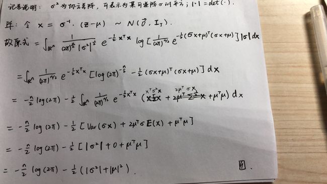
  ∫qθ(z)logpθ(z)dz=∫N(z;μ,σ2)logN(z;0,I)dz=−J2log(2π)−12∑j=1J(μ2j+σ2j) ∫ q θ ( z ) log ⁡ p θ ( z ) d z = ∫ N ( z ; μ , σ 2 ) log ⁡ N ( z ; 0 , I ) d z = − J 2 log ⁡ ( 2 π ) − 1 2 ∑ j = 1 J ( μ j 2 + σ j 2 )

  And:
  

  ∫qθ(z)logqθ(z)dz=∫N(z;μ,σ2)logN(z;μ,σ2)dz=−J2log(2π)−12∑j=1J(1+logσ2j) ∫ q θ ( z ) log ⁡ q θ ( z ) d z = ∫ N ( z ; μ , σ 2 ) log ⁡ N ( z ; μ , σ 2 ) d z = − J 2 log ⁡ ( 2 π ) − 1 2 ∑ j = 1 J ( 1 + log ⁡ σ j 2 )

  Therefore:
  

  −DKL(qϕ(z)∥pθ(z))=∫qθ(z)(logpθ(z)−logqθ(z))dz=12∑j=1L(1+log(σi2j)−μi2j−σi2j) − D K L ( q ϕ ( z ) ∥ p θ ( z ) ) = ∫ q θ ( z ) ( log ⁡ p θ ( z ) − log ⁡ q θ ( z ) ) d z = 1 2 ∑ j = 1 L ( 1 + log ⁡ ( σ j i 2 ) − μ j i 2 − σ j i 2 )

  此处附上相关证明：
  

  Visulization

  Since the prior of the latent space is Gaussian, linearly spaced coordinates on the unit square were transformed through the inverse CDF of the Gaussian to produce values of the latent variables $z$.