【图像处理】Bilinear Image Scaling
Bilinear image scaling is about the same as nearest neighbor image scaling except with interpolation. Instead of copying the neighboring pixels (which often results in jaggy image), interpolation technique based on surrounding pixels is used to produce much smoother scaling.
Although bilinear scaling is not exactly complicated, it is a composite algorithm based on other more basic function. As the name might have suggested, the algorithm is a combination of two linear interpolations. It is not mandatory to know what linear interpolation is but doing is not really that bad. I suggest the reader to follow through at least the brief explanation.
Linear Interpolation (a brief explanation)
Linear interpolation is a method to estimate an arbitrary point between two other points. Consider two points of colors on a canvas, red and green. Imagine a straight line between the dots, and somewhere on this imaginary line put a new dot. What is a suitable color for this new dot? Any color is fine really, but we are talking about interpolation so we should be doing that. Putting our little imaginary line in perspective,

Figure 1: What is a suitable color for Y?
In this illustration, a yet unknown color dot Y is placed somewhere between A (red) and B (green). Other only known thing is the distance between A and B which is L and the distance between A and Y which is l. This information is sufficient to construct the so called linear interpolation function.

Figure 2: Linear interpolation equation
This function will be able to tell what Y's color is. If you are interested to know the expected color for Y, check the full article for Linear Interpolation.
Texture
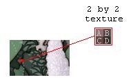
Going back to the original topic, the other trivial but still important term is the texture. This is not about the whole image itself but only a small portion of it. In the simplest of bilinear scaling, the usual texture dimension is only two by two, a texture containing only four pixels. The illustration below should help with getting the idea for this,

Figure3: 2 by 2 texture
That small texture with A, B, C, and D is what we are talking about. Keep in mind there will be many smaller textures like this composing the entire image. This also means the algorithm has many smaller textures to work with.
The algorithm
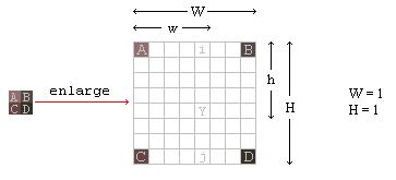
Scaling an image goes in two ways, making it larger or to make it smaller. By enlarging an image, some new pixels are constructed by means of interpolation. By shrinking, we are tempted to think the right pixels are selected to keep while the others are thrown away, but this is not the case. Unlike nearest neighbor shrinking where pixels are thrown, bilinear shrinking estimates a smaller resolution of the original image. Even though details are lost, almost all the new pixels in the shrunk image do not come directly from their original, but interpolated, indirectly keeping the properties of lost pixels. It should be understood this is not always the case, shrinking image to half size (and smaller) significantly reduce image quality – not much different from nearest neighbor shrinking. This also applies to sizing up more than double the original size.

Figure4:Enlarged image introduces "white spaces"
For the purpose of this article, explanation will follow the making-it-larger path because that is probably why people are reading this anyway. So we start by enlarging a small texture such as shown in figure 4. Note: this is not to be mistaken as a requirement to enlarge every single texture found in an image. The objective is finding the colors for all white spaces, including i, j, and Y. Here linear interpolation comes into play, first find the relation between A, i, and B. Using linear interpolation function that we derived at the beginning (figure 2), we get this equation,

Do the same for C, j, and D and we get,

Now we have two linear interpolation equations. Next is to combine the two equations forming a single equation that is called the bilinear function.

Substituting equation 1 and 2 into 3 we get,

Using this last equation, all white spaces can now be interpolated!! That's it!!
Implementation
Yeah right. Putting the idea on paper is all nice and convenient but actually doing it is an entirely different thing. This time we discuss how a basic implementation is worked out.
Two things must be understood before we proceed, first is the actual code for scaling the image. Secondly is the code for interpolation process. These two are distinct, the first as mentioned is for the enlargement and at the same time introducing all the white spaces. The second part which is the interpolation process decides the color for these white spaces. Nearest neighbor algorithm share similar code for scaling, just missing the interpolation part.
Here is a Java snippet for 1 channel (grayscale) bilinear image scaling. Each pixel is an int and has a range from 0 to 255.
/*

 * Bilinear resize grayscale image.

 * pixels is an array of size w * h.

 * Target dimension is w2 * h2.

 * w2 * h2 cannot be zero.

 *

 * @param pixels Image pixels.

 * @param w Image width.

 * @param h Image height.

 * @param w2 New width.

 * @param h2 New height.

 * @return New array with size w2 * h2.

 */

public int[] resizeBilinearGray(int[] pixels, int w, int h, int w2, int h2) {

    int[] temp = new int[w2*h2] ;

    int A, B, C, D, x, y, index, gray ;

    float x_ratio = ((float)(w-1))/w2 ;

    float y_ratio = ((float)(h-1))/h2 ;

    float x_diff, y_diff, ya, yb ;

    int offset = 0 ;

    for (int i=0;i<h2;i++) {

        for (int j=0;j<w2;j++) {

            x = (int)(x_ratio * j) ;

            y = (int)(y_ratio * i) ;

            x_diff = (x_ratio * j) - x ;

            y_diff = (y_ratio * i) - y ;

            index = y*w+x ;


            // range is 0 to 255 thus bitwise AND with 0xff

            A = pixels[index] & 0xff ;

            B = pixels[index+1] & 0xff ;

            C = pixels[index+w] & 0xff ;

            D = pixels[index+w+1] & 0xff ;


            // Y = A(1-w)(1-h) + B(w)(1-h) + C(h)(1-w) + Dwh

            gray = (int)(

                    A*(1-x_diff)*(1-y_diff) +  B*(x_diff)*(1-y_diff) +

                    C*(y_diff)*(1-x_diff)   +  D*(x_diff*y_diff)

                    ) ;


            temp[offset++] = gray ;

        }

    }

    return temp ;

}
Here is a Java snippet for 4 channels (color) bilinear image scaling. Each pixel is a packed int containing alpha, red, green, and blue information.
/*

 * Bilinear resize ARGB image.

 * pixels is an array of size w * h.

 * Target dimension is w2 * h2.

 * w2 * h2 cannot be zero.

 *

 * @param pixels Image pixels.

 * @param w Image width.

 * @param h Image height.

 * @param w2 New width.

 * @param h2 New height.

 * @return New array with size w2 * h2.

 */

public int[] resizeBilinear(int[] pixels, int w, int h, int w2, int h2) {

    int[] temp = new int[w2*h2] ;

    int a, b, c, d, x, y, index ;

    float x_ratio = ((float)(w-1))/w2 ;

    float y_ratio = ((float)(h-1))/h2 ;

    float x_diff, y_diff, blue, red, green ;

    int offset = 0 ;

    for (int i=0;i<h2;i++) {

        for (int j=0;j<w2;j++) {

            x = (int)(x_ratio * j) ;

            y = (int)(y_ratio * i) ;

            x_diff = (x_ratio * j) - x ;

            y_diff = (y_ratio * i) - y ;

            index = (y*w+x) ;

            a = pixels[index] ;

            b = pixels[index+1] ;

            c = pixels[index+w] ;

            d = pixels[index+w+1] ;


            // blue element

            // Yb = Ab(1-w)(1-h) + Bb(w)(1-h) + Cb(h)(1-w) + Db(wh)

            blue = (a&0xff)*(1-x_diff)*(1-y_diff) + (b&0xff)*(x_diff)*(1-y_diff) +

                   (c&0xff)*(y_diff)*(1-x_diff)   + (d&0xff)*(x_diff*y_diff);


            // green element

            // Yg = Ag(1-w)(1-h) + Bg(w)(1-h) + Cg(h)(1-w) + Dg(wh)

            green = ((a>>8)&0xff)*(1-x_diff)*(1-y_diff) + ((b>>8)&0xff)*(x_diff)*(1-y_diff) +

                    ((c>>8)&0xff)*(y_diff)*(1-x_diff)   + ((d>>8)&0xff)*(x_diff*y_diff);


            // red element

            // Yr = Ar(1-w)(1-h) + Br(w)(1-h) + Cr(h)(1-w) + Dr(wh)

            red = ((a>>16)&0xff)*(1-x_diff)*(1-y_diff) + ((b>>16)&0xff)*(x_diff)*(1-y_diff) +

                  ((c>>16)&0xff)*(y_diff)*(1-x_diff)   + ((d>>16)&0xff)*(x_diff*y_diff);


            temp[offset++] =

                    0xff000000 | // hardcode alpha

                    ((((int)red)<<16)&0xff0000) |

                    ((((int)green)<<8)&0xff00) |

                    ((int)blue) ;

        }

    }

    return temp ;

}
Caveat
Bilinear scaling performs best when the desired output dimension is no more than double or half its original size. If that is the case however, it might be good to implement additional technique called Mip Mapping on top of the existing algorithm.