ML | SVM

What's xxx

An SVM model is a representation of the examples as points in space, mapped so that the examples of the separate categories are divided by a clear gap that is as wide as possible. New examples are then mapped into that same space and predicted to belong to a category based on which side of the gap they fall on.

In addition to performing linear classification, SVMs can efficiently perform a non-linear classification using what is called the kernel trick, implicitly mapping their inputs into high-dimensional feature spaces.  The transformation may be nonlinear and the transformed space high dimensional; thus though the classifier is a hyperplane in the high-dimensional feature space, it may be nonlinear in the original input space.

Classifying data is a common task in machine learning. Suppose some given data points each belong to one of two classes, and the goal is to decide which class a new data point will be in. In the case of support vector machines, a data point is viewed as a p-dimensional vector (a list of p numbers), and we want to know whether we can separate such points with a (p − 1)-dimensional hyperplane. This is called a linear classifier. We choose the hyperplane so that the distance from it to the nearest data point on each side is maximized. If such a hyperplane exists, it is known as the maximum-margin hyperplane and the linear classifier it defines is known as a maximum margin classifier. 

Any hyperplane can be written as the set of points $\mathbf{x}$ satisfying
$\mathbf{w}\cdot\mathbf{x} - b=0,\,$
where $\cdot$ denotes the dot product and ${\mathbf{w}}$ the (not necessarily normalized) normal vector to the hyperplane.

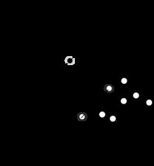
Maximum-margin hyperplane and margins for an SVM trained with samples from two classes. Samples on the margin are called the support vectors.

It was converted into a quadratic programming optimization problem. The solution can be expressed as a linear combination of the training vectors

$\mathbf{w} = \sum_{i=1}^n{\alpha_i y_i\mathbf{x_i}}.$
Only a few $\alpha_i$ will be greater than zero. The corresponding $\mathbf{x_i}$ are exactly the support vectors, which lie on the margin and satisfy $y_i(\mathbf{w}\cdot\mathbf{x_i} - b) = 1$. From this one can derive that the support vectors also satisfy

$\mathbf{w}\cdot\mathbf{x_i} - b = 1 / y_i = y_i \iff b = \mathbf{w}\cdot\mathbf{x_i} - y_i$
which allows one to define the offset b. In practice, it is more robust to average over all $N_{SV}$ support vectors:

$b = \frac{1}{N_{SV}} \sum_{i=1}^{N_{SV}}{(\mathbf{w}\cdot\mathbf{x_i} - y_i)}$

Writing the classification rule in its unconstrained dual form reveals that the maximum-margin hyperplane and therefore the classification task is only a function of the support vectors, the subset of the training data that lie on the margin.

Using the fact that $\|\mathbf{w}\|^2 = \mathbf{w}\cdot \mathbf{w}$ and substituting $\mathbf{w} = \sum_{i=1}^n{\alpha_i y_i\mathbf{x_i}}$, one can show that the dual of the SVM reduces to the following optimization problem:

Maximize (in $\alpha_i$ )

$\tilde{L}(\mathbf{\alpha})=\sum_{i=1}^n \alpha_i - \frac{1}{2}\sum_{i, j} \alpha_i \alpha_j y_i y_j \mathbf{x}_i^T \mathbf{x}_j=\sum_{i=1}^n \alpha_i - \frac{1}{2}\sum_{i, j} \alpha_i \alpha_j y_i y_j k(\mathbf{x}_i, \mathbf{x}_j)$
subject to (for any $i = 1, \dots, n$)

$\alpha_i \geq 0,\, $
and to the constraint from the minimization in $b$

$\sum_{i=1}^n \alpha_i y_i = 0.$
Here the kernel is defined by $k(\mathbf{x}_i,\mathbf{x}_j)=\mathbf{x}_i\cdot\mathbf{x}_j.$

$W$ can be computed thanks to the $\alpha$ terms:

$\mathbf{w} = \sum_i \alpha_i y_i \mathbf{x}_i.$