1. Those sorting algorithms with the property that the sorted order they determine is based only on comparisons between the input elements are called comparison sorts.
2. Any comparison sort must make Ω(n lg n) comparisons in the worst case to sort n elements. Thus, merge sort and heapsort are asymptotically optimal, and no comparison sort exists that is faster by more than a constant factor.
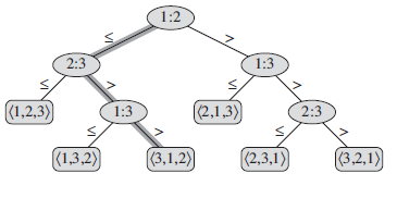
3. We can view comparison sorts abstractly in terms of decision trees. A decision tree is a full binary tree that represents the comparisons between elements that are performed by a particular sorting algorithm operating on an input of a given size:
In a decision tree, we annotate each internal node by i :j for some i and j in the
range 1≤i,j≤n, where n is the number of elements in the input sequence. We
also annotate each leaf by a permutation <π(1), π(2), ... , π(n)>. The execution of the sorting algorithm corresponds to tracing a simple path from the root of the decision tree down to a leaf. Each internal node indicates a comparison and when we come to a leaf, the sorting algorithm has established the ordering (aπ(1) ≤ aπ(2) ≤ ... ≤ aπ(n) ). Because any correct sorting algorithm must be able to produce each permutation of its input, each of the n! permutations on n elements must appear as one of the leaves of the decision tree for a comparison sort to be correct. The length of the longest simple path from the root of a decision tree to any of its reachable leaves ( the height of the tree ) represents the worst-case number of comparisons that the corresponding sorting algorithm performs. Suppose a decision tree with height h has l reachable leaves, then n! ≤ l ≤ 2^h , so h ≥ lg(n!) = Ω(n lg n).
4. Counting sort assumes that each of the n input elements is an integer in the range 0 to k, for some integer k. When k = O(n), the sort runs in θ(n) time.
5. Counting sort determines, for each input element x, the number of elements less than x. It uses this information to place element x directly into its position in the output array:
// sort n elements whose value is non-negative integers and less than max using couting sort
	int[] countingSort(int[] input , int max) {
		int[] counting = new int[max]; // by default initialized to 0

		for ( int i = 0 ; i < input.length ; i ++ ) {
			// don't check whether each number is really less than k
			counting[input[i]] ++;
		}
		// after above processing counting[i] indicates the number of input elements equal to i
		for ( int i = 1 ; i < max ; i ++) {
			counting[i] += counting[i-1];
		}
		// after above processing counting[i] indicates the number of input elements less than or equal to i

		int[] output = new int[input.length];
		for ( int i = input.length - 1 ; i >= 0  ; i --) {
			int element = input[i];
			// if there are 10 elements less than or equal to the current element (including itself), than it should be put into the position 9
			output[--counting[element]] = element;
		}

		return output;
	}
6. An important property of counting sort is that it is stable: numbers with the same value appear in the output array in the same order as they do in the input array. The property of stability is important only when satellite data are carried around with the element being sorted.
7. Radix sort sorts on the least significant digit first using a stable sort. Then it sorts the entire numbers again on the second-least significant digit. The process continues
until the numbers have been sorted on all d digits.
8. We sometimes use radix sort to sort records of information that are keyed by multiple fields.
9. With counting sort as the intermediate stable sort, Radix sort will run in θ(d(n+k)) time assuming each digit is less than k and each number has at most d digits. If d and k are not too large, then the algorithm will run in θ(n) time.
10. Given n b-bit numbers and any positive integer r ≤ b, radix sort correctly sorts these numbers in θ((b/r)(n+2^r)) time if the stable sort it uses takes θ(n+k) time for inputs in the range 0 to k. Because we can view each number as having d = ⌈b/r⌉digits of r bits each. Each digit is an integer in the range 0 to 2^r-1, so that we can use counting sort with k=2^r-1. If b < ⌊lg n⌋, then for any value of r ≤ b, we have that (n + 2^r ) = θ(n). Thus, choosing r = b yields a running time of (b/b)(n+2^b) = θ(n), which is asymptotically optimal. If b ≥ lg(n), then choosing r =⌊lg n⌋ gives the best time to within a constant factor.
11. Quicksort often uses hardware caches more effectively than radix sort.
12. Bucket sort assumes that the input is drawn from a uniform distribution and has an average-case running time of O(n).
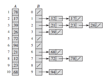
13. Bucket sort assumes that the input is generated by a random process that distributes elements uniformly and independently over the interval [0, 1). Bucket sort divides the interval [0, 1) into n equal-sized subintervals, or buckets, and then distributes the n input numbers into the buckets. Since the inputs are uniformly and independently distributed over [0, 1), we do not expect many numbers to fall into each bucket. To produce the output, we simply sort the numbers in each bucket and then go through the buckets in order, listing the elements in each.
// sort n elements whose value is uniformly distributed among [0,1) using bucket sorting
	double[] bucketSorting(double[] input) {
		ArrayList<Double>[] buckets = new ArrayList[input.length];

		// initialize the buckets
		for (int i = 0; i < input.length; i ++) {
			buckets[i] = new ArrayList<Double>();
		}

		//allocate each element to its corresponding bucket
		for ( int i = 0 ; i < input.length; i ++) {
			double element = input[i];
			buckets[ (int) (element * input.length)].add(element);
		}

		// concatenating the buckets after sorting
		for ( int i = 0 , j = 0; i < input.length ; i ++) {
			ArrayList<Double> bucket = buckets[i];
			Collections.sort(bucket);
			for (double element : bucket) {
				input[j++] = element;
			}
		}

		return input;


	}
14. Even if the input is not drawn from a uniform distribution, bucket sort may still run in linear time as long as the input has the property that the sum of the squares of the bucket sizes is linear in the total number of elements.


