Machine Learning - VII. Regularization规格化 (Week 3)

http://blog.csdn.net/pipisorry/article/details/43966361

机器学习Machine Learning - Andrew NG courses学习笔记

Regularization 规格化

The Problem of Overfitting过拟合问题

linear regression example线性规划的例子(housing prices)

underfit(or the hypothesis having high bias; figure1): if the algorithmhas a very strong preconception, or a very strong bias that housing prices are going to vary linearly with their size and despite the data to the contrary.

overfit(figure3): The term high variance is a historical or technical one.But, the intuition is that,if we're fitting such a high order polynomial, then, the hypothesis can fit almost any function and this face of possible hypothesis is just too large, it's too variable.

And we don't have enough data to constrain it to give us a good hypothesis so that's called overfitting.the curve tries too hard to fit the training set, so that it even fails to generalize to new examples and fails to predict prices on new examples.

logistic regression example with two features X1 and x2逻辑规划的例子(breast tumor cancer)

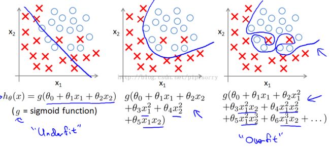
just_right(figure2):  add to your features these quadratic terms,you could get a decision boundary that might look more like figure 2.And that's a pretty good fit to the data.
overfit(figure3): try really hard to find a decision boundary that fits your training data or go to great lengths to contort(扭曲) itself,to fit every single training example well.
Addressing overfitting解决过拟合问题

In the previous examples, we had one or two dimensional data so,we could just plot the hypothesis and see what was going on and select the appropriate degree polynomial.

But that doesn't always work.And, in fact more often we may have learning problems that where we just have a lot of features.And there is not just a matter of selecting what degree polynomial.it also becomes much harder to plot the data and it becomes much harder to visualize it,to decide what features to keep or not.

All of these features seem kind of useful.But, if we have a lot of features, and, very little training data, then, over fitting can become a problem.

解决方法

disadvantage：throwing away some of the features, is also throwing away some of the information you have about the problem.

 怎么检测underfit & overfit?

Debugging and diagnosing things that can go wrong with learning algorithms

【Advice for Applying Machine Learning-鉴别两种类型的问题】

Cost Function代价函数

直觉上的解释

规格化的好处

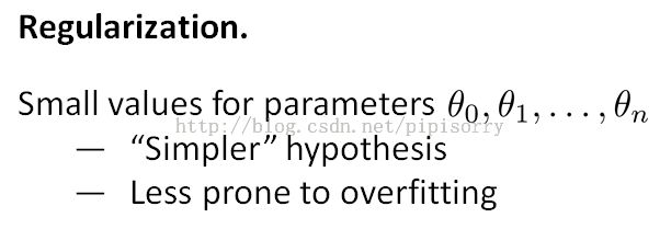
Note: it is possible to show that having smaller values of the parameters corresponds to usually smoother functions as well for the simpler.And it is kind of hard to explain unless you implement yourself and see it for yourself.

But the example of having theta 3 and theta 4 be small gave us a simpler hypothesis helps explain why, at least give some intuition as to why this might be true.

规格化cost function

regularization term: 规格化项

1. at the end to shrink every single parameter theta 1-100.
2. That sort of the convention that,the sum I equals one through N, rather than I equals zero through N. whether you include,theta zero or not, in practice, make very little difference to the results.


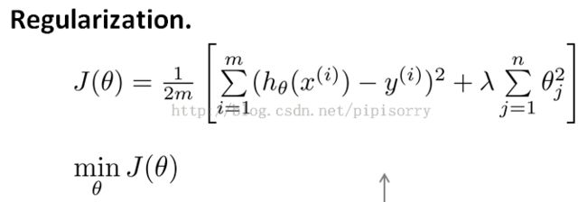
regularization parameter: lambda,controls the trade of between the goal of fitting the training set well and the goal of keeping the parameter plan small and therefore keeping the hypothesis relatively simple to avoid overfitting.
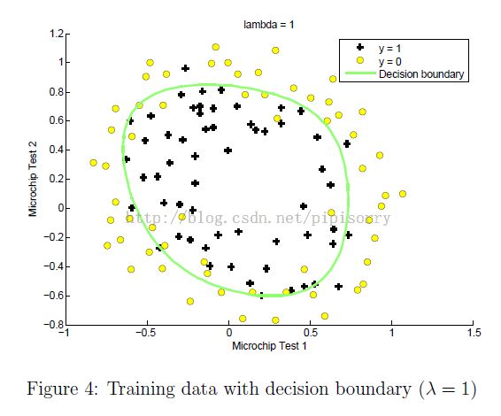
you can get out in fact a curve that isn't quite a quadratic function, but is much smoother and much simpler and maybe a curve like the magenta line that,gives a much better hypothesis for this data.

regularization parameter: lambda设置太大带来的问题

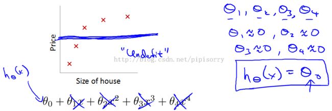
if the regularization parameter monitor is set to be very large,then what will happen is we will end up penalizing the parameters very highly.Then we end up with all of these parameters close to zero,that is akin to fitting a flat horizontal straight line to the data,this is an example of underfitting.

lambda设置的影响在mlclass-ex2  -  2.5 Optional (ungraded) exercises中的一个例子

parameter lambda怎么自动选择？

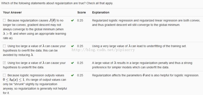
参见： 【X. Advice for Applying Machine Learning- Regularization and Bias_Variance规格化和偏差_方差】



Regularized Linear Regression规格化线性规划

For linear regression, we had worked out two learning algorithms,gradient descent and the normal equation.
There we take those two algorithms and generalize them to the case of regularized linear regression.

Gradient descent解线性规划的改进

Note:

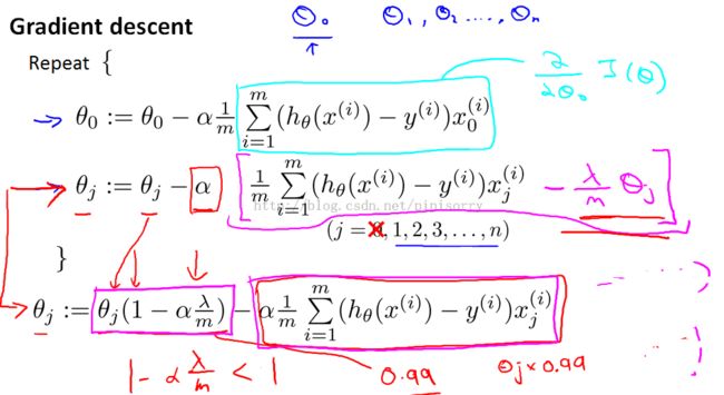
theta zero单独分开原因：for our regularized linear regression,we don't penalize theta zero.so treating theta zero slightly differently.
的效果： theta J times 0.99 has the effect of shrinking theta J a little bit towards 0.this makes theta J a bit smaller.
regularized的解释： when using regularized linear regression what we're doing is on every regularization were multiplying data J by a number that is a little bit less than one, so we're shrinking the parameter a little bit, and then we're performing a similar update as before.
Normal equation解线性规划的改进

推导： using the new definition of J of theta, with the regularization objective.Then this new formula for theta is the one that will give you the global minimum of J of theta.？？？

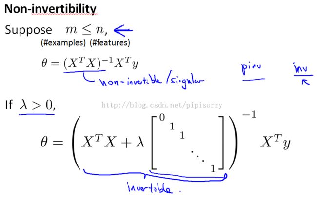
Note: so long as the regularization parameter is strictly greater than zero.It is actually possible to prove that this matrix X transpose X plus parameter time, this matrix will not be singular and that this matrix will be invertible.

Regularized Logistic Regression规格化逻辑规划

overfitting的可能由来：More generally if you have logistic regression with a lot of features.Not necessarily polynomial ones, but just with a lot of features you can end up with overfitting.

规格化Gradient descent方法

（注意:中括号里应该是+lambda/m*thetaj）

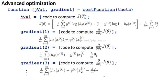
规格化高级方法

Code for regularized logistic regression

1. code to compute the regularized cost function:

J = -1/m * (y' * log(sigmoid(X*theta)) + (1-y)' * log(1 - sigmoid(X*theta))) + lambda/(2*m) * (theta'*theta - theta(1)*theta(1));

2. code to compute the gradient of the regularized  cost:

1>        #vectorized,推荐

grad = 1/m*(X'*(sigmoid(X*theta)-y));
temp = theta;temp(1)=0;
grad = grad+lambda/m*temp;

2>       #vectorized

tmp = X' * (sigmoid(X * theta) - y);
grad = (tmp + lambda * theta) / m;
grad(1) = tmp(1) / m; 

3>        #non-vectorized

grad(1) = 1/m*(sigmoid(X*theta)-y)'*X(:,1);
for i=2:size(theta)
    grad(i) = 1/m*(sigmoid(X*theta)-y)'*X(:,i) + lambda/m*theta(i);

end

Note:

end keyword in indexing:One special keyword you can use in indexing is the end keyword in indexing.This allows us to select columns (or rows) until the end of the matrix.
For example, A(:, 2:end) will only return elements from the 2nd to last column of A. Thus, you could use this together with the sum and .^ operations to compute the sum of only the elements you are interested in(e.g., sum(z(2:end).^2)).

Review复习

More:

Whereas linear regression, logistic regression, you can form polynomial terms, but it turns out that there are much more powerful nonlinear quantifiers that can then sort of polynomial regression.

更多非线性分类器的学习在后面的讲解中，而不是使用linear\logistic regression的高维feature来实现。如神经网络Neural Networks、支持向量机SVM。

from:http://blog.csdn.net/pipisorry/article/details/43966361