UVa OJ 199 - Partial differential equations (偏微分方程)
Time limit: 3.000 seconds
限时:3.000秒
Problem
问题
In engineering sciences, partial differential equations play an important and central role. For example, the temperature of a metal plate can be expressed as a partial differential equation if the temperature on the boundaries is known. This is called a boundary value problem.
在工程技术领域,偏微分方程扮演了重要的中心角色。比方说,如果已知一块金属板边界上的温度,那么整块金属板的温度就可由一个偏微分方程表示,这称为边值问题。
Usually, it is not easy to solve these problems. Analytical solutions exist only in very special cases. But there are some more or less "good" numerical ways to solve boundary value problems.
一般来说,解这些偏微分方程是很困难的,仅在一些特定的条件下才会存在解析解。但是仍有或多或少的一些“好”的数值方法来解决边值问题。
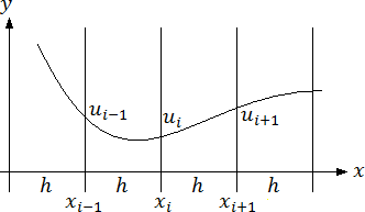
We now will look at one method which works with finite difference approximations for the derivatives of a function. For this approach, we do not look at an analytical function u(x) but we are only interested in the values of u at a finite set of discrete points xi : ui=u(xi). The distance between two adjacent points, xi and xi+1, is constant: h=xi+1–xi(cf. figure 1).
我们现在来看一个使用有限差分逼近对方程求导的方法。在这个方法中,分析方程u(x)不是重点,我们需要关心的是在一个有限离散点集xi:ui=u(xi)中u的值。两个相邻点xi和xi+1之间的距离是一个常量:h=xi+1–xi(见图1)。

Figure 1: u(x) at some discrete points xi
图1:u(x)在一些离散点xi处的值
The finite difference approximation of a first derivative of the function u(x) is
函数u(x)的一阶导的有限差分逼近为:
 (1)
(1)
The second derivative is approximated by
二阶导的逼近为:
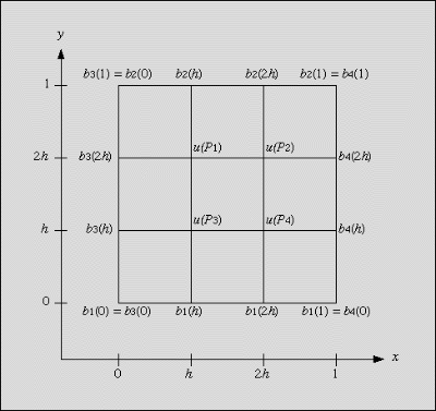
This approximation works with 2-dimensional functions u(x,y) as well. For simplicity we only work on square problems, i.e. (x, y) is element of [0, 1]×[0, 1]. Again, the area of the function is discretized in a similar way: xi+1–xi=yi+1–yi=h=1/n, for some integer n≥2. We only look at the values of u(x,y) at the discrete points Pk=(xi, yi):ui,j=u(Pk). With this discretization, we have a function ui,j as shown in figure 2:
该逼近方法也同样适用于2元方程u(x,y)。简单起见,我们只考虑正方形的情况,即(x, y)都是[0, 1]×[0, 1]中的一个元素。对函数所在的区域也进行类似的离散化:xi+1–xi=yi+1–yi=h=1/n(n≥2,且n为整数)。我们看到u(x,y)在离散点Pk处的值Pk=(xi, yi):ui,j=u(Pk)。离散化以后,我们得到了图2显示的方程ui,j:
 Figure 2: Function ui,j in the discretization area
图2:在离散区域内的函数ui,j
On the boundary, u(xi, yi) is given by 4 known functions:
在边界上,u(xi, yi)为4个已知的函数:
- u(xi, 0) = b1(xi)
- u(xi, 1) = b2(xi)
- u(0, yj) = b3(yj)
- u(1, yj) = b4(yj) (3)
The points Pk cover the inner points of the discretization area, i.e. the area without the boundary. They are numbered from left to right and from top to bottom like English text.
设点Pk为离散化区域内部的任意点,即区域内除边界外的点。这些点从左至右,从上至下进行编号,类似于文章的书写顺序。
What we now want to do is to solve the poisson-equation in the area [0, 1]×[0, 1]:
我们现在需要做的是按照上面给出的边界条件,在[0, 1]×[0, 1]这个区域内求解泊松方程:
with the above boundary conditions. f(x,y) is a given 2-dimensional function. With equation (2) and the above discretization, the poisson-equation can be approximated at
f(x,y)是一个给定的二元函数。根据方程式(2)和上面的离散化,泊松方程可以逼近为:
 (5)
(5)
where fi,j is the function f(x,y), evaluated at the discrete points (xi, yj).
式中fi,j就是函数f(x,y)在离散点(xi, yj)处的值。
Formula (5) can be written in a more readable form, depending on the position of the discrete points:
方程(5)还可以按照离散点的位置写成更容易读懂的形式:
A similar equation, which we will use as an example below, is:
下面就是一个类似的方程,我们用它来作为例子:
We call the 3×3 matrix on the left hand side v and the 3×3 matrix on the right hand side g.
我们把左边的3×3矩阵称为v,把右边3×3的矩阵称为g。
Now, equation (6b) can be formulated in every point of the discrete area of figure 2:
现在,方程(6b)在图2中的任何一个离散点都可以写成如下的公式:
and (7) is a linear equation system for the values of u(x,y) at the points P1, P2, P3 and P4.
(7)式是一个u(x,y)在P1、P2、P3和P4点处值的线性方程组。
By rearranging and adding the terms on each line, the linear equation system can be formulated as:
对各行方程进行整理和添项后,线性方程组可以由如下公式表示:
- az = b (8)
where a is a 4×4 matrix and b is a vector with 4 elements. Vector z represents the unknown values of u(x,y) at the points P1, P2, P3 and P4.
式中a是一个4×4的矩阵,b是一个由4个元素的向量。向量z表示未知数:u(x,y)在点P1、P2、P3和P4处的值。
You are to write a program that creates the linear equation system (7) in the form (8) for any two matrices v and g (6). As input, the two matrices v and g and the functions b1, b2, b3, b4, and f are given. Also, a parameter n is given as the number of discretization intervals. Thus, h=1/n. As the result, your program should calculate the matrix a and the vector b. For this more general case, there are (n-1)2 inner points and a and b must be sized accordingly.
你要写一个程序,对给定的任意矩阵v和g(6),以(8)式的格式建立线性方程组(7)。v和g两个矩阵以及函数b1、b2、b3、b4和f都在输入中给定。同样,离散点的间隔值将以参数n给出,即h=1/n。你的程序应计算出矩阵a和向量b作为结果。在更一般的情况下,将存在(n-1)2个内部点,并且a和b必须符合相应的大小。
Input
输入
The input file consists of m tests. The number m is given in the first line of the file. The first line of each test contains the number n which gives the number of discretizations intervals as defined above. You may assume that 2≤n≤30. Then the 3×3 matrices v and g follow. The following four lines contain the functions b1, b2, b3 and b4, each given as a vector of order n+1, containing the values for 0, h, 2h, ..., 1. Finally, the function f is given as a n+1 by n+1 matrix. Like the vectors before, it contains the values for x,y=0, h, 2h, ..., 1. Each row contains from left to right the function values for increasing x values while each column contains from top to bottom the function values for decreasing y values.
输入的数据包括m组测试用例(以下简称用例),m的值在数据的第1行给出。每组用例的第一行为上面定义的离散化间隔值n。你可以认为2≤n≤30。下面是3×3的矩阵v和g。接下来的4行为函数b1、b2、 b3和b4,每个函数都由一组n+1阶的向量给出,包括0,h,2h,...,1的值。最后,函数f由n+1乘n+1的矩阵给出。类似于上面的向量,它也包含x,y=0, h, 2h, ..., 1的值。每行函数值对应的自变量x的值从左至右依次增大,每列对应的自变量y的值从上到下依次减小。
A vector occupies one line. Its values are given in ascending order, separated by a space. A n by n matrix occupies n lines. Its rows are given in ascending order as vectors, which occupy one line each. All values found in the input file are integer values.
每个向量独占一行,其值顺序给出,每两个值之间有一个空格。一个n乘n的矩阵占n行,各行亦顺序给出,并各独占一行输出。输入数据中给出的所有值均为整数。
Output
输出
For each test found in the input file, your program should output the matrices a and b. Matrix a is a (n–1)2×(n–1)2 matrix (the discretization area (cf. figure 2) contains (n–1)2 inner points, which are unknown). The vector b is of order (n–1)2. They should be output in the same format as the vectors and matrices in the input file. Your output should only contain integer values. Note that the expression 1/h2 yields an integer number and that all other calculations can also be done using integer numbers.
对应于输入数据中的每个用例,你的程序应输出矩阵a和b。矩阵a是一个(n–1)2×(n–1)2的矩阵(离散化区域(见图2)包括个(n–1)2内部点,其值均为未知数)。向量b是(n–1)2阶的。应该按照输入数据中的矩阵和向量的格式输出结果。你的程序应该只包括矩形值。注意表达式1/h2的值应该是整数,且所有计算都应该用整数来完成。
Sample Input
输入示例
1
3
1 0 2
0 -4 0
3 0 4
0 5 0
6 0 7
0 8 0
3 4 5 6
0 1 2 3
3 2 1 0
6 5 4 3
1 1 1 1
2 2 2 2
3 3 3 3
4 4 4 4
Sample Output
输出示例
-36 0 0 36
0 -36 27 0
0 18 -36 0
9 0 0 -36
-35 -188 -189 -315
Analysis
分析
这是一道非常忽悠人的题,千万别被标题和题目的描述吓倒。这题其实和偏微分方程根本没有任何关系,甚至和矩阵、行列式的计算也没啥关系,就是一个二维数组的顺序填充,算法非常简单。题目的主要意图是要计算一个线性的多元一次方程组。最后虽然说让求出未知数,但输出部分却明确告知:只要给出系数矩阵和常数向量就可以了,不用继续进行矩阵乘法求出未知数。对照图2、(6b)式和(7)式,很快就知道怎么填充了。如果屏幕不够大,建议画在一页纸上看,方便对照。
下面代码中的r数组为要求的b向量,其它数组名称与题目所给的一样。i和j分别循环内部离散区域的行和列,s和t分别循环每一个点周围3×3子矩阵的行和列,也没啥好注释的,一看便知。
Solution
解析
#include <algorithm>
#include <iostream>
#include <string>
#include <vector>
using namespace std;
//主函数
int main(void) {
	int m, n, v[3][3], g[3][3], b[4][31], f[31][31], *a = new int[841 * 841];
	for (cin >> m; --m >= 0; ) {
		cin >> n;
		int r[841] = {0}, nSize = (n - 1) * (n - 1), h2 = n * n;
		for (int i = 0; i < 3; ++i) {
			for (int j = 0; j < 3; cin >> v[i][j++]);
		}
		for (int i = 0; i < 3; ++i) {
			for (int j = 0; j < 3; cin >> g[i][j++]);
		}
		for (int i = 0; i < 4; ++i) {
			for (int j = 0; j < n + 1; cin >> b[i][j++]);
		}
		for (int i = 0; i < n + 1; ++i) {
			for (int j = 0; j < n + 1; cin >> f[i][j++]);
		}
		for (int i = 1; i < n; ++i) {
			for (int j = 1; j < n; ++j) {
				int id = (i - 1) * (n - 1) + j - 1;
				for (int s = 0; s < 3; ++s) {
					for (int t = 0; t < 3; ++t) {
						int as = i + s - 1, at = j + t - 1;
						r[id] += f[as][at] * g[s][t];
						if (as == 0) {
							r[id] -= b[1][at] * v[s][t] * h2;
						}
						else if (at == 0) {
							r[id] -= b[2][n - as] * v[s][t] * h2;
						}
						else if (as == n) {
							r[id] -= b[0][at] * v[s][t] * h2;
						}
						else if (at == n) {
							r[id] -= b[3][n - as] * v[s][t] * h2;
						}
						else {
							int aid = (as - 1) * (n - 1) + at - 1;
							a[id * nSize + aid] = v[s][t] * h2;
						}
					}
				}
			}
		}
		for (int i = 0; i < nSize; ++i) {
			for (int j = 0; j < nSize - 1; ++j) {
				cout << a[i * nSize + j] << ' ';
			}
			cout << a[i * nSize + nSize - 1] << endl;
		}
		for (int i = 0; i < nSize - 1; ++i) {
			cout << r[i] << ' ';
		}
		cout << r[nSize - 1] << endl;
	}
	delete[] a;
	return 0;
}
