【Matlab】关于Matlab的一些代码片段

转载，请保持连接：http://blog.csdn.net/stalendp/article/details/44904639

这篇文章收集关于Matlab的一些代码片段，以便查阅：

function [] = myFunc(n)
    t = 0:0.001:2;
    y = myFunc0(t, n);
    figure;
    plot(t, y);
end

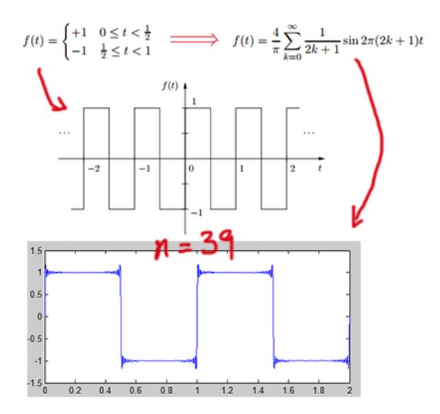
% 方波
function [ y ] = myFunc0( t, n )
rt = 0;
for k = 0:n
    rt = rt + sin(2*pi*(2*k+1)*t)/(2*k+1);
end
y = rt * 4 / pi;
end

方波图如下：

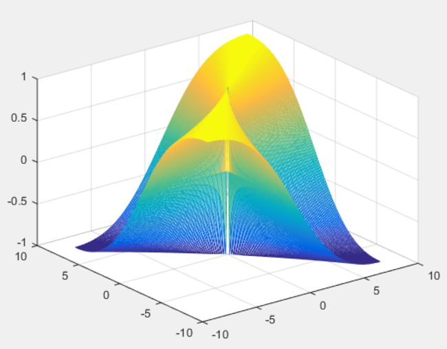
2) 打印3D曲面：

 [x,y] = meshgrid(-8:.1:8);
 z = (2.*x.*y)./(x.*x + y.*y);
mesh(x,y,z);

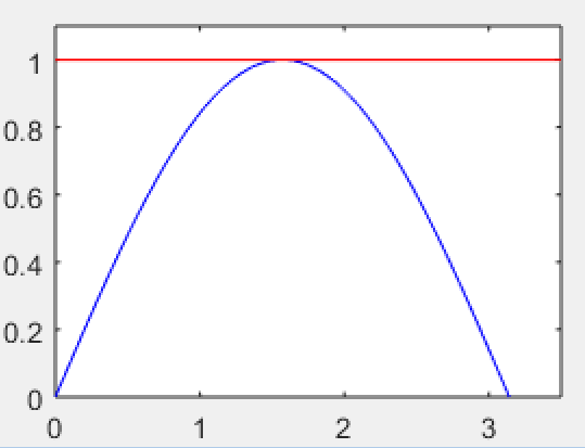
3. 一些打印技巧：

% example 1
x = linspace(0,pi);
y = sin(x);
ymax = max(y);
figure(1)
plot(x, y, '-b')
hold on
plot(xlim, [1 1]*ymax, '-r')
hold off
axis([xlim    0  1.1])

% example 2
x = linspace(0,5,1000);
y = sin(100*x)./exp(x);
ax1 = subplot(2,1,1);
plot(x,y)

ax2 = subplot(2,1,2);
plot(x,y)
xlim(ax2,[0 1])

 

4. 函数的一些使用技巧（function handler， anonymous function); 可以使用matlab中的类来 更好的管理函数模块，请参考5中的方法

function study(n)
    sqr = @(nn) nn.^2;
    C = {@e1, @e2, @e3, @e4, @() sqr(3)};
    C{n}()
end

%相关快捷键：Ctrl+R, Ctrl+T, Ctrl+I %{ %}
function e1
    disp('This is example1');
    figure(1)
    x = linspace(0,pi);
    y = sin(x);
    ymax = max(y);
    plot(x, y, '-b')
    hold on
    plot(xlim, [1 1]*ymax, '-r')
    hold off
    axis([xlim    0  1.1])
end

function e2
    disp('This is example2');
    figure(2)
    x = linspace(0,5,1000);
    y = sin(100*x)./exp(x);
    ax1 = subplot(2,1,1);
    plot(x,y)

    ax2 = subplot(2,1,2);
    plot(x,y)
    xlim(ax2,[0 1])
end

function e3
    disp('This is example3');
    figure(3)
    [x,y] = meshgrid(-8:.1:8);  
    z = (2.*x.*y)./(x.*x + y.*y);  
    mesh(x,y,z);      
end

function e4
    disp('This is example4');
    figure(4)
    myFunc(20);
end

5. 用类的方式来管理函数模块

classdef myclass
    properties
    end
    
    methods
        function e1(obj)
            disp('This is example1');
            figure(1)
            x = linspace(0,pi);
            y = sin(x);
            ymax = max(y);
            plot(x, y, '-b')
            hold on
            plot(xlim, [1 1]*ymax, '-r')
            hold off
            axis([xlim    0  1.1])
        end
        
        function e2(obj)
            disp('This is example2');
            figure(2)
            x = linspace(0,5,1000);
            y = sin(100*x)./exp(x);
            ax1 = subplot(2,1,1);
            plot(x,y)
            
            ax2 = subplot(2,1,2);
            plot(x,y)
            xlim(ax2,[0 1])
        end
        
        function e3(obj)
            disp('This is example3');
            figure(3)
            [x,y] = meshgrid(-8:.1:8);
            z = (2.*x.*y)./(x.*x + y.*y);
            mesh(x,y,z);
        end
        
        function e4(obj)
            disp('This is example4');
            figure(4)
            myFunc(20);
        end
    end
end

6. 当然matlab还有非常赞的publish功能，请参考： Publishing MATLAB Code from The Editor

7. 高分辨率下，matlab自动改变分辨率的bug的解决方案：Matlab Changes reslution after opening simulink 

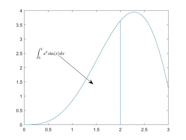
8.用LaTeX来输出公式; 更多公式符号请参考：https://en.wikibooks.org/wiki/LaTeX/Mathematics

8-1）积分公式

x = linspace(0,3);
y = x.^2.*sin(x);
plot(x,y)
line([2,2],[0,2^2*sin(2)])
str = '$$ \int_{0}^{2} x^2\sin(x) dx $$';
text(0.25,2.5,str,'Interpreter','latex')
annotation('arrow','X',[0.32,0.5],'Y',[0.6,0.4])

8-2) 求和公式

x = linspace(-3,3);
y = sin(x);
plot(x,y)

y0 = x;
hold on
plot(x,y0)

y1 = x - x.^3/6;
plot(x,y1)
hold off
str = '$$\sin(x) = \sum_{n=0}^{\infty}{\frac{(-1)^n x^{2n+1}}{(2n+1)!}}$$';
%             text(-2,1,str,'Interpreter','latex')
title(str,'Interpreter','latex');

9. Matlab字体设置； home->preference->Fonts； 推荐字体：雅黑、Consolas、Mono；其中Mono、Consolas都不支持中文，可以用和雅黑的结合体(点击链接可以转到下载页面)：雅黑+Mono, 雅黑+Consolas;  
另外，介绍一篇关于编程字体的文章：有哪些适合用于写代码的西文字体？

10. 漂亮地输出公式：

A = sym(pascal(2));
B = eig(A);
pretty(B)

// 结果如下：
/ 3   sqrt(5) \
| - - ------- |
| 2      2    |
|             |
| sqrt(5)   3 |
| ------- + - |
\    2      2 /

11. Matlab打印矩阵的LaTeX的获取：

A = [1 2 3; 4 5 6; 7 8 9];
latex_table = latex(sym(A))

输出结果为：

12. pretty 和 LaTeX输出的区别：

同样一个矩阵，可以在控制台输出（用pretty），也可以在plot窗口或者publish页面（用LateX）显示。

用11中的矩阵做例子：

%% 测试 pretty 和 LaTeX
A = [1 2 3; 4 5 6; 7 8 9];

% pretty 代码
pretty(sym(A));

% plot 代码：
str = ['$$', latex(sym(A)), '$$'];
title(str ,'Interpreter','latex')