BP神经网络Python实现

作者：金良（[email protected]） csdn博客：http://blog.csdn.net/u012176591

训练数据

某地区20年公路运量数据

年份	人口数量/万人	机动车数量/万辆	公路面积/万平方千米	公路客运量/万人	公路货运量/万吨
1990	20.55	0.6	0.09	5126	1237
1991	22.44	0.75	0.11	6217	1379
1992	25.37	0.85	0.11	7730	1385
1993	27.13	0.90	0.14	9145	1399
1994	29.45	1.05	0.20	10460	1663
1995	30.1	1.35	0.23	11387	1714
1996	30.96	1.45	0.23	12353	1834
1997	34.06	1.60	0.32	15750	4322
1998	36.42	1.70	0.32	18304	8132
1999	38.09	1.85	0.34	19836	8936
2000	39.13	2.15	0.36	21024	11099
2001	39.99	2.20	0.36	19490	11203
2002	41.93	2.25	0.38	20433	10524
2003	44.59	2.35	0.49	22598	11115
2004	47.30	2.50	0.56	25107	13320
2005	52.89	2.60	0.59	33442	16762
2006	55.73	2.70	0.59	36836	18673
2007	56.76	2.85	0.67	40548	20724
2008	59.17	2.95	0.69	42927	20803
2009	60.63	3.10	0.79	43462	21804

人工神经网络源码

import numpy as np
import matplotlib.pyplot as plt

def logsig(x):
    return 1/(1+np.exp(-x))

#人数(单位：万人)
population=[20.55,22.44,25.37,27.13,29.45,30.10,30.96,34.06,36.42,38.09,39.13,39.99,41.93,44.59,47.30,52.89,55.73,56.76,59.17,60.63]
#机动车数(单位：万辆)
vehicle=[0.6,0.75,0.85,0.9,1.05,1.35,1.45,1.6,1.7,1.85,2.15,2.2,2.25,2.35,2.5,2.6,2.7,2.85,2.95,3.1]
#公路面积(单位：万平方公里)
roadarea=[0.09,0.11,0.11,0.14,0.20,0.23,0.23,0.32,0.32,0.34,0.36,0.36,0.38,0.49,0.56,0.59,0.59,0.67,0.69,0.79]
#公路客运量(单位：万人)
passengertraffic=[5126,6217,7730,9145,10460,11387,12353,15750,18304,19836,21024,19490,20433,22598,25107,33442,36836,40548,42927,43462]
#公路货运量(单位：万吨)
freighttraffic=[1237,1379,1385,1399,1663,1714,1834,4322,8132,8936,11099,11203,10524,11115,13320,16762,18673,20724,20803,21804]

samplein = np.mat([population,vehicle,roadarea]) #3*20
sampleinminmax = np.array([samplein.min(axis=1).T.tolist()[0],samplein.max(axis=1).T.tolist()[0]]).transpose()#3*2，对应最大值最小值
sampleout = np.mat([passengertraffic,freighttraffic])#2*20
sampleoutminmax = np.array([sampleout.min(axis=1).T.tolist()[0],sampleout.max(axis=1).T.tolist()[0]]).transpose()#2*2，对应最大值最小值

#3*20
sampleinnorm = (2*(np.array(samplein.T)-sampleinminmax.transpose()[0])/(sampleinminmax.transpose()[1]-sampleinminmax.transpose()[0])-1).transpose()
#2*20
sampleoutnorm = (2*(np.array(sampleout.T).astype(float)-sampleoutminmax.transpose()[0])/(sampleoutminmax.transpose()[1]-sampleoutminmax.transpose()[0])-1).transpose()

#给输出样本添加噪音
noise = 0.03*np.random.rand(sampleoutnorm.shape[0],sampleoutnorm.shape[1])
sampleoutnorm += noise




maxepochs = 60000
learnrate = 0.035
errorfinal = 0.65*10**(-3)
samnum = 20
indim = 3
outdim = 2
hiddenunitnum = 8

w1 = 0.5*np.random.rand(hiddenunitnum,indim)-0.1
b1 = 0.5*np.random.rand(hiddenunitnum,1)-0.1
w2 = 0.5*np.random.rand(outdim,hiddenunitnum)-0.1
b2 = 0.5*np.random.rand(outdim,1)-0.1

errhistory = []

for i in range(maxepochs):
    hiddenout = logsig((np.dot(w1,sampleinnorm).transpose()+b1.transpose())).transpose()
    networkout = (np.dot(w2,hiddenout).transpose()+b2.transpose()).transpose()
    err = sampleoutnorm - networkout
    sse = sum(sum(err**2))

    errhistory.append(sse)
    if sse < errorfinal:
        break

    delta2 = err

    delta1 = np.dot(w2.transpose(),delta2)*hiddenout*(1-hiddenout)

    dw2 = np.dot(delta2,hiddenout.transpose())
    db2 = np.dot(delta2,np.ones((samnum,1)))

    dw1 = np.dot(delta1,sampleinnorm.transpose())
    db1 = np.dot(delta1,np.ones((samnum,1)))

    w2 += learnrate*dw2
    b2 += learnrate*db2

    w1 += learnrate*dw1
    b1 += learnrate*db1




# 误差曲线图
errhistory10 = np.log10(errhistory)
minerr = min(errhistory10)
plt.plot(errhistory10)
plt.plot(range(0,i+1000,1000),[minerr]*len(range(0,i+1000,1000)))

ax=plt.gca()
ax.set_yticks([-2,-1,0,1,2,minerr])
ax.set_yticklabels([u'$10^{-2}$',u'$10^{-1}$',u'$1$',u'$10^{1}$',u'$10^{2}$',str(('%.4f'%np.power(10,minerr)))])
ax.set_xlabel('iteration')
ax.set_ylabel('error')
ax.set_title('Error History')
plt.savefig('errorhistory.png',dpi=700)
plt.close()


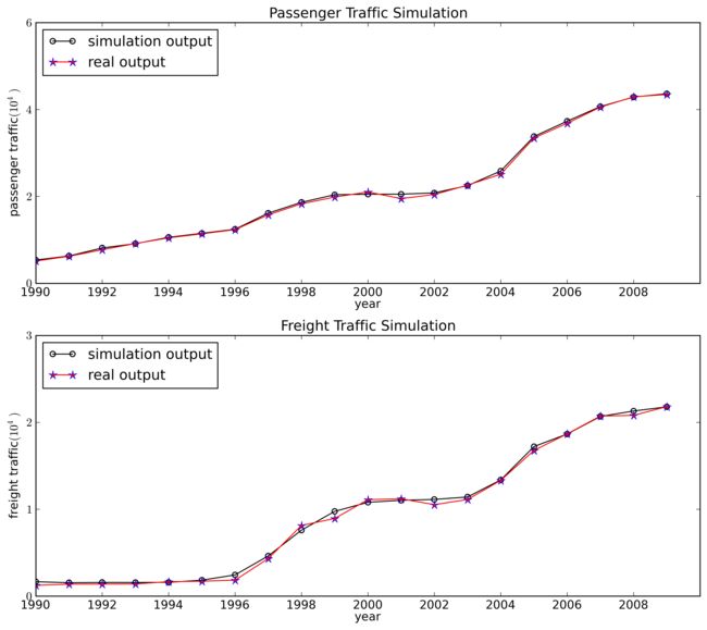
# 仿真输出和实际输出对比图
hiddenout = logsig((np.dot(w1,sampleinnorm).transpose()+b1.transpose())).transpose()
networkout = (np.dot(w2,hiddenout).transpose()+b2.transpose()).transpose()
diff = sampleoutminmax[:,1]-sampleoutminmax[:,0]
networkout2 = (networkout+1)/2
networkout2[0] = networkout2[0]*diff[0]+sampleoutminmax[0][0]
networkout2[1] = networkout2[1]*diff[1]+sampleoutminmax[1][0]

sampleout = np.array(sampleout)

fig,axes = plt.subplots(nrows=2,ncols=1,figsize=(12,10))
line1, =axes[0].plot(networkout2[0],'k',marker = u'$\circ$')
line2, = axes[0].plot(sampleout[0],'r',markeredgecolor='b',marker = u'$\star$',markersize=9)

axes[0].legend((line1,line2),('simulation output','real output'),loc = 'upper left')

yticks = [0,20000,40000,60000]
ytickslabel = [u'$0$',u'$2$',u'$4$',u'$6$']
axes[0].set_yticks(yticks)
axes[0].set_yticklabels(ytickslabel)
axes[0].set_ylabel(u'passenger traffic$(10^4)$')

xticks = range(0,20,2)
xtickslabel = range(1990,2010,2)
axes[0].set_xticks(xticks)
axes[0].set_xticklabels(xtickslabel)
axes[0].set_xlabel(u'year')
axes[0].set_title('Passenger Traffic Simulation')

line3, = axes[1].plot(networkout2[1],'k',marker = u'$\circ$')
line4, = axes[1].plot(sampleout[1],'r',markeredgecolor='b',marker = u'$\star$',markersize=9)
axes[1].legend((line3,line4),('simulation output','real output'),loc = 'upper left')
yticks = [0,10000,20000,30000]
ytickslabel = [u'$0$',u'$1$',u'$2$',u'$3$']
axes[1].set_yticks(yticks)
axes[1].set_yticklabels(ytickslabel)
axes[1].set_ylabel(u'freight traffic$(10^4)$')

xticks = range(0,20,2)
xtickslabel = range(1990,2010,2)
axes[1].set_xticks(xticks)
axes[1].set_xticklabels(xtickslabel)
axes[1].set_xlabel(u'year')
axes[1].set_title('Freight Traffic Simulation')

fig.savefig('simulation.png',dpi=500,bbox_inches='tight')
plt.close()

训练效果图