OpenCV3的人脸检测－使用Python

OpenCV3的对象检测－使用Python

http://docs.opencv.org/master/d7/d8b/tutorial_py_face_detection.html

Goal

In this session,

• We will see the basics of face detection using Haar Feature-based Cascade Classifiers

• We will extend the same for eye detection etc.
  
  

使用 Haar 分类器进行面部检测

目标:

• 以 Haar 特征分类器为基础的面部检测技术。

• 将面部检测扩展到眼部检测等。

Basics

Object Detection using Haar feature-based cascade classifiers is an effective object detection method proposed by Paul Viola and Michael Jones in their paper, "Rapid Object Detection using a Boosted Cascade of Simple Features" in 2001. It is a machine learning based approach where a cascade function is trained from a lot of positive and negative images. It is then used to detect objects in other images.

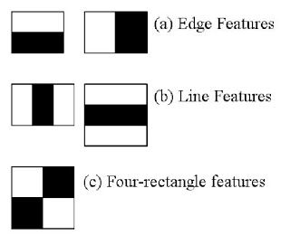
Here we will work with face detection. Initially, the algorithm needs a lot of positive images (images of faces) and negative images (images without faces) to train the classifier. Then we need to extract features from it. For this, haar features shown in below image are used. They are just like our convolutional kernel. Each feature is a single value obtained by subtracting sum of pixels under white rectangle from sum of pixels under black rectangle.

1 基础

以 Haar 特征分类器为基础的对象检测技术是一种非常有效的对象检测 技术(2001 年 Paul_Viola 和 Michael_Jones 提出)。它是基于机器学习的, 通过使用大量的正负样本图像训练得到一个 cascade_function,最后再用它 来做对象检测。

现在我们来学习面部检测。开始时,算法需要大量的正样本图像(面部图 像)和负样本图像(不含面部的图像)来训练分类器。我们需要从其中提取特 征。下图中的 Haar 特征会被使用。它们就像我们的卷积核。每一个特征是一 个值,这个值等于黑色矩形中的像素值之后减去白色矩形中的像素值之和。

Now all possible sizes and locations of each kernel is used to calculate plenty of features. (Just imagine how much computation it needs? Even a 24x24 window results over 160000 features). For each feature calculation, we need to find sum of pixels under white and black rectangles. To solve this, they introduced the integral images. It simplifies calculation of sum of pixels, how large may be the number of pixels, to an operation involving just four pixels. Nice, isn't it? It makes things super-fast.

使用所有可能的核来计算足够多的特征。(想象一下这需要多少计算量?仅 仅是一个 24x24 的窗口就有 160000 个特征)。对于每一个特征的计算我们 好需要计算白色和黑色矩形内的像素和。为了解决这个问题,作者引入了积分 图像,这可以大大的简化求和运算,对于任何一个区域的像素和只需要对积分 图像上的四个像素操作即可。非常漂亮,它可以使运算速度飞快!

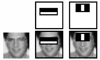
But among all these features we calculated, most of them are irrelevant. For example, consider the image below. Top row shows two good features. The first feature selected seems to focus on the property that the region of the eyes is often darker than the region of the nose and cheeks. The second feature selected relies on the property that the eyes are darker than the bridge of the nose. But the same windows applying on cheeks or any other place is irrelevant. So how do we select the best features out of 160000+ features? It is achieved by Adaboost.

但是在我们计算得到的所有的这些特征中,大多数是不相关的。如下图所 示。上边一行显示了两个好的特征,第一个特征看上去是对眼部周围区域的描 述,因为眼睛总是比鼻子黑一些。第二个特征是描述的是眼睛比鼻梁要黑一些。但是如果把这两个窗口放到脸颊的话,就一点都不相关。那么我们怎样从超过160000+ 个特征中选出最好的特征呢?使用 Adaboost。

For this, we apply each and every feature on all the training images. For each feature, it finds the best threshold which will classify the faces to positive and negative. But obviously, there will be errors or misclassifications. We select the features with minimum error rate, which means they are the features that best classifies the face and non-face images. (The process is not as simple as this. Each image is given an equal weight in the beginning. After each classification, weights of misclassified images are increased. Then again same process is done. New error rates are calculated. Also new weights. The process is continued until required accuracy or error rate is achieved or required number of features are found).

为了达到这个目的,我们将每一个特征应用于所有的训练图像。对于每一 个特征,我们要找到它能够区分出正样本和负样本的最佳阈值。但是很明显, 这会产生错误或者错误分类。我们要选取错误率最低的特征,这说明它们是检 测面部和非面部图像最好的特征。(这个过程其实不像我们说的这么简单。在开 始时每一张图像都具有相同的权重,每一次分类之后,被错分的图像的权重会 增大。同样的过程会被再做一遍。然后我们又得到新的错误率和新的权重。重 复执行这个过程知道到达要求的准确率或者错误率或者要求数目的特征找到)。

Final classifier is a weighted sum of these weak classifiers. It is called weak because it alone can't classify the image, but together with others forms a strong classifier. The paper says even 200 features provide detection with 95% accuracy. Their final setup had around 6000 features. (Imagine a reduction from 160000+ features to 6000 features. That is a big gain).

最终的分类器是这些弱分类器的加权和。之所以成为弱分类器是应为只是 用这些分类器不足以对图像进行分类,但是与其他的分类器联合起来就是一个 很强的分类器了。文章中说 200 个特征就能够提供 95% 的准确度了。他们最 后使用 6000 个特征。(从 160000 减到 6000,效果显著呀!)。

So now you take an image. Take each 24x24 window. Apply 6000 features to it. Check if it is face or not. Wow.. Wow.. Isn't it a little inefficient and time consuming? Yes, it is. Authors have a good solution for that.

现在你有一幅图像,对每一个 24x24 的窗口使用这 6000 个特征来做检 查,看它是不是面部。这是不是很低效很耗时呢?的确如此,但作者有更好的 解决方法。

In an image, most of the image region is non-face region. So it is a better idea to have a simple method to check if a window is not a face region. If it is not, discard it in a single shot. Don't process it again. Instead focus on region where there can be a face. This way, we can find more time to check a possible face region.

在一副图像中大多数区域是非面部区域。所以最好有一个简单的方法来证 明这个窗口不是面部区域,如果不是就直接抛弃,不用对它再做处理。而不是 集中在研究这个区域是不是面部。按照这种方法我们可以在可能是面部的区域 多花点时间。

For this they introduced the concept of Cascade of Classifiers. Instead of applying all the 6000 features on a window, group the features into different stages of classifiers and apply one-by-one. (Normally first few stages will contain very less number of features). If a window fails the first stage, discard it. We don't consider remaining features on it. If it passes, apply the second stage of features and continue the process. The window which passes all stages is a face region. How is the plan !!!

Authors' detector had 6000+ features with 38 stages with 1, 10, 25, 25 and 50 features in first five stages. (Two features in the above image is actually obtained as the best two features from Adaboost). According to authors, on an average, 10 features out of 6000+ are evaluated per sub-window.

So this is a simple intuitive explanation of how Viola-Jones face detection works. Read paper for more details or check out the references in Additional Resources section.

为了达到这个目的作者提出了级联分类器的概念。不是在一开始就对窗口 进行这 6000 个特征测试,将这些特征分成不同组。在不同的分类阶段逐个使 用。(通常前面很少的几个阶段使用较少的特征检测)。如果一个窗口第一阶段 的检测都过不了就可以直接放弃后面的测试了,如果它通过了就进入第二阶段 的检测。如果一个窗口经过了所有的测试,那么这个窗口就被认为是面部区域。 这个计划是不是很帅!!

作者将 6000 多个特征分为 38 个阶段,前五个阶段的特征数分别为 1,10,25,25 和 50。(上图中的两个特征其实就是从 Adaboost 获得的最好 特征)。

According to authors, on an average, 10 features out of 6000+ are evaluated per sub-window.

上面是我们对 Viola-Jones 面部检测是如何工作的直观解释。读一下原始 文献或者更多资源中非参考文献将会对你有更大帮助。

Haar-cascade Detection in OpenCV

OpenCV comes with a trainer as well as detector. If you want to train your own classifier for any object like car, planes etc. you can use OpenCV to create one. Its full details are given here: Cascade Classifier Training.

Here we will deal with detection. OpenCV already contains many pre-trained classifiers for face, eyes, smile etc. Those XML files are stored in opencv/data/haarcascades/ folder. Let's create face and eye detector with OpenCV.

First we need to load the required XML classifiers. Then load our input image (or video) in grayscale mode.

2 OpenCV 中的 Haar 级联检测

OpenCV 自带了训练器和检测器。如果你想自己训练一个分类器来检测 汽车,飞机等的话,可以使用 OpenCV 构建。其中的细节在这里:Cascade Classifier Training

现在我们来学习一下如何使用检测器。OpenCV 已经包含了很多已经训练 好的分类器,其中包括:面部,眼睛,微笑等。这些 XML 文件保存在/opencv/ data/haarcascades/文件夹中。下面我们将使用 OpenCV 创建一个面部和眼 部检测器。

首先我们要加载需要的 XML 分类器。然后以灰度格式加载输入图像或者 是视频。

# -*- coding: utf-8 -*-
import numpy as npimport cv2
face_cascade = cv2.CascadeClassifier('haarcascade_frontalface_default.xml')
eye_cascade = cv2.CascadeClassifier('haarcascade_eye.xml')
img = cv2.imread('sachin.jpg')
gray = cv2.cvtColor(img, cv2.COLOR_BGR2GRAY)

Now we find the faces in the image. If faces are found, it returns the positions of detected faces as Rect(x,y,w,h). Once we get these locations, we can create a ROI for the face and apply eye detection on this ROI (since eyes are always on the face !!! ).

现在我们在图像中检测面部。如果检测到面部,它会返回面部所在的矩形 区域 Rect(x,y,w,h)。一旦我们获得这个位置,我们可以创建一个 ROI 并在 其中进行眼部检测。(谁让眼睛长在脸上呢!)

#Detects objects of different sizes in the input image.

# The detected objects are returned as a list of rectangles. 
#cv2.CascadeClassifier.detectMultiScale(image, scaleFactor, 
minNeighbors, flags, minSize, maxSize) #scaleFactor – Parameter 
specifying how much the image size is reduced at each image
#scale.

#minNeighbors – Parameter specifying how many neighbors each candidate rectangle should
#have to retain it.
#minSize – Minimum possible object size. Objects smaller than that are ignored.
#maxSize – Maximum possible object size. Objects larger than that are ignored.
faces = face_cascade.detectMultiScale(gray, 1.3, 5)
for (x,y,w,h) in faces:
           img = cv2.rectangle(img,(x,y),(x+w,y+h),(255,0,0),2)
           roi_gray = gray[y:y+h, x:x+w]
           roi_color = img[y:y+h, x:x+w]
           eyes = eye_cascade.detectMultiScale(roi_gray)
           for (ex,ey,ew,eh) in eyes: 
               cv2.rectangle(roi_color,(ex,ey),(ex+ew,ey+eh),(0,255,0),2)

cv2.imshow('img',img)
cv2.waitKey(0)
cv2.destroyAllWindows()

Result looks like below:

结果如下:

更多资源

1. Video Lecture on Face Detection and Tracking

2. AninterestinginterviewregardingFaceDetectionbyAdamHar- vey