有限体积PDE求解器--基于Python的FiPy

http://www.ctcms.nist.gov/fipy/index.html

• NIST Home > 
• MML > 
• CTCMS > 
•  FiPy >

FiPy: A Finite Volume PDE Solver Using Python
Version 3.1

Cahn-Hilliard

Phase Field

Level Set

Questions? Suggestions?

Join the mailing list

Recent mailing list traffic recorded at GMANE (links leave NIST): 

You can also open an issue at thetracker.

Quick search

 

Enter search terms or a module, class or function name.

Contact

FiPy developers
Jonathan Guyer
Daniel Wheeler
James Warren

Join our mailing list

100 Bureau Drive, M/S 6555
Gaithersburg, MD 20899

301-975-5329 Telephone
301-975-4553 Facsimile

FiPy: A Finite Volume PDE Solver Using Python

FiPy is an object oriented, partial differential equation (PDE) solver, written in Python, based on a standard finite volume (FV) approach. The framework has been developed in the Materials Science and Engineering Division (MSED) and Center for Theoretical and Computational Materials Science (CTCMS), in the Material Measurement Laboratory (MML) at the National Institute of Standards and Technology (NIST).

The solution of coupled sets of PDEs is ubiquitous to the numerical simulation of science problems. Numerous PDE solvers exist, using a variety of languages and numerical approaches. Many are proprietary, expensive and difficult to customize. As a result, scientists spend considerable resources repeatedly developing limited tools for specific problems. Our approach, combining the FV method and Python, provides a tool that is extensible, powerful and freely available. A significant advantage to Python is the existing suite of tools for array calculations, sparse matrices and data rendering.

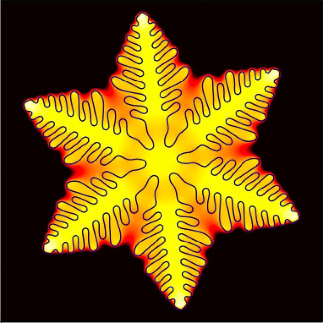
The FiPy framework includes terms for transient diffusion, convection and standard sources, enabling the solution of arbitrary combinations of coupled elliptic, hyperbolic and parabolic PDEs. Currently implemented models include phase field [BoettingerReview:2002] [ChenReview:2002] [McFaddenReview:2002] treatments of polycrystalline, dendritic, and electrochemical phase transformations as well as a level set treatment of the electrodeposition process[NIST:damascene:2001].

If you use FiPy in your research, please cite: (bibtex) (endnote) (pdf)

J. E. Guyer, D. Wheeler & J. A. Warren, "FiPy: Partial Differential Equations with Python," Computing in Science & Engineering 11(3) pp. 6—15 (2009), doi:10.1109/MCSE.2009.52, http://www.ctcms.nist.gov/fipy

Documentation

About FiPy start here Installation how to install FiPy on different platforms FiPy Usage how to use FiPy Examples examples of usage FAQs frequently asked questions (with answers!) License terms of use

Numerical Approach background on numerical solutions to PDEs FiPy Design FilosoPhy of FiPy FiPy API reference for Python programmers Credits significant contributors Publications papers and talks about (or using) FiPy

Applications

Superconformal Electrodeposition level set treatment of "Damascene" electrodeposition

Virtual Kinetics of Materials Laboratory interactive graphical examples from Purdue University

FiPy@MatForge

Download Source Code

wiki Reporting Bugs

Indices and tables

Global Module Index quick access to all modules General Index all functions, classes, terms Glossary the most important terms explained

Search Page search this documentation Complete Table of Contents lists all sections and subsections References lists of source materials

一个求解Cahn-Hilliard方程的实例:

http://www.ctcms.nist.gov/fipy/examples/cahnHilliard/generated/examples.cahnHilliard.mesh2D.html

examples.cahnHilliard.mesh2D

The spinodal decomposition phenomenon is a spontaneous separation of an initially homogenous mixture into two distinct regions of different properties (spin-up/spin-down, component A/component B). It is a “barrierless” phase separation process, such that under the right thermodynamic conditions, any fluctuation, no matter how small, will tend to grow. This is in contrast to nucleation, where a fluctuation must exceed some critical magnitude before it will survive and grow. Spinodal decomposition can be described by the “Cahn-Hilliard” equation (also known as “conserved Ginsberg-Landau” or “model B” of Hohenberg & Halperin)

where  is a conserved order parameter, possibly representing alloy composition or spin. The double-well free energy function  penalizes states with intermediate values of  between 0 and 1. The gradient energy term , on the other hand, penalizes sharp changes of . These two competing effects result in the segregation of  into domains of 0 and 1, separated by abrupt, but smooth, transitions. The parameters  and determine the relative weighting of the two effects and  is a rate constant.

We can simulate this process in FiPy with a simple script:

>>> from fipy import *

(Note that all of the functionality of NumPy is imported along with FiPy, although much is augmented for FiPy‘s needs.)

>>> if __name__ == "__main__":
...     nx = ny = 1000
... else:
...     nx = ny = 20
>>> mesh = Grid2D(nx=nx, ny=ny, dx=0.25, dy=0.25)
>>> phi = CellVariable(name=r"$\phi$", mesh=mesh)

We start the problem with random fluctuations about 

>>> phi.setValue(GaussianNoiseVariable(mesh=mesh,
...                                    mean=0.5,
...                                    variance=0.01))

FiPy doesn’t plot or output anything unless you tell it to:

>>> if __name__ == "__main__":
...     viewer = Viewer(vars=(phi,), datamin=0., datamax=1.)

For FiPy, we need to perform the partial derivative  manually and then put the equation in the canonical form by decomposing the spatial derivatives so that each Term is of a single, even order:

FiPy would automatically interpolate D * a**2 * (1 - 6 * phi * (1 - phi)) onto the faces, where the diffusive flux is calculated, but we obtain somewhat more accurate results by performing a linear interpolation from phi at cell centers to PHI at face centers. Some problems benefit from non-linear interpolations, such as harmonic or geometric means, and FiPy makes it easy to obtain these, too.

>>> PHI = phi.arithmeticFaceValue
>>> D = a = epsilon = 1.
>>> eq = (TransientTerm()
...       == DiffusionTerm(coeff=D * a**2 * (1 - 6 * PHI * (1 - PHI)))
...       - DiffusionTerm(coeff=(D, epsilon**2)))

Because the evolution of a spinodal microstructure slows with time, we use exponentially increasing time steps to keep the simulation “interesting”. The FiPy user always has direct control over the evolution of their problem.

>>> dexp = -5
>>> elapsed = 0.
>>> if __name__ == "__main__":
...     duration = 1000.
... else:
...     duration = 1000.

>>> while elapsed < duration:
...     dt = min(100, numerix.exp(dexp))
...     elapsed += dt
...     dexp += 0.01
...     eq.solve(phi, dt=dt, solver=LinearLUSolver())
...     if __name__ == "__main__":
...         viewer.plot()
...     elif (max(phi.globalValue) > 0.7) and (min(phi.globalValue) < 0.3) and elapsed > 10.:
...         break

>>> print (max(phi.globalValue) > 0.7) and (min(phi.globalValue) < 0.3)
True

The National Institute of Standards and Technology (NIST) is an agency of the U.S. Department of Commerce