1.该算法的主要思想是:根据现有数据对分类边界线建立回归公式,以此分类(二值分类、也称概率分类)。这里的回归指的最佳拟合,表示要找到最佳的参数集,训练的过程就是寻找最佳参数的过程。
2.logistic回归算法(适用数值型和标称型数据)
优点:计算代价不高,容易理解和计算。
缺点:欠拟合,分类精度可能不高。
3.激活函数sigmoid函数是一种阶跃函数,输出范围在[0,1],在回归问题中,我们需要找到最佳的回归系数,需要用到最优化算法:如梯度上升(求最大值)或是梯度下降(求最小值),求梯度要求在定义的点上有定义且可微,在梯度迭代过程中总能使我们找到最佳的路径。
梯度下降算法
w=w−α▽f(w)
梯度上升算法
w=w+α▽f(w)
4.梯度下降(上升)算法每次更新回归系数都要遍历整个数据集,而随机梯度下降(上升)算法是梯度下降算法的改进型,一次只用一个样本来更新回归系数,由于可以在新的样本到来时对分类器进行增量式更新,因此随机梯度算法是一个在线学习算法。
5.数据处理时,若遇到缺失值时的处理办法
- 使用可用特征的时均值来填补缺失值
- 使用特殊值来填充,如-1
- 忽略缺失值的样本
- 使用相似的样本均值来填补缺失值
- 使用机器学习的算法来预测缺失值
6.例子1:logistic+梯度上升算法
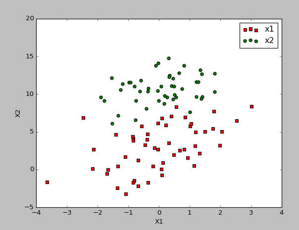
6.1有一个简单的数据集合(数据和代码在本文下面给出),数据有两个特征x1,x2,如下图中所示,有两类分别是红色和绿色部分所示,下面我们要通过logistic回归的方法将这两类分出来
6.3.首先建立一个logistic.py的文件,这个文件主要是写我们所要实现的函数
import numpy as np
import matplotlib.pyplot as plt
def loadDataSet():
dataMat = []
labelMat = []
fr = open('testSet.txt')
for line in fr.readlines():
lineArr = line.strip().split()
dataMat.append([1.0, float(lineArr[0]), float(lineArr[1])])
labelMat.append(int(lineArr[2]))
return dataMat, labelMat
def sigmoid(inX):
return 1.0/(1+np.exp(-inX))
def gradAscent(dataMatIn, classLabels):
dataMat = np.mat(dataMatIn)
labelMat = np.mat(classLabels).T
m,n = np.shape(dataMat)
alpha = 0.001
maxCycles = 600
weights = np.ones((n,1))
for k in xrange(maxCycles):
h = sigmoid(dataMat*weights)
error = (labelMat-h)
weights = weights+alpha*dataMat.T*error
return weights
6.4,建立一个main.py的文件,在这个文件中调用函数
import numpy as np
import logistic as reg
dataArr,labelMat = reg.loadDataSet()
weights = reg.gradAscent(dataArr, labelMat)
weights = weights.getA()
print weights
得到如下权重
[[ 4.44558222] [ 0.50711996] [-0.6573892 ]]
logistic.py的代码中h = sigmoid(dataMat*weights)中dataMat是向量,最后h也是向量,这种方法是便利整个数据集合,对已100个左右的样本来说可以,但数据量大时,这种计算方法会占用过多和资源,计算效率低,后面会有将具体的优化算法:随机梯度上升算法,下面来拟合我们的数据,画出决策边界。在logistic.py文件中继续添加下面代码
def plotBestFit(weights):
dataMat,labelMat = loadDataSet()
dataArr = np.array(dataMat)
n = np.shape(dataArr)[0]
xcord1 = []
ycord1 = []
xcord2 = []
ycord2 = []
for i in range(n):
if int(labelMat[i]) ==1:
xcord1.append(dataArr[i,1])
ycord1.append(dataArr[i,2])
else:
xcord2.append(dataArr[i,1])
ycord2.append(dataArr[i,2])
fig =plt.figure()
ax = fig.add_subplot(111)
ax.scatter(xcord1,ycord1,s=30,c='red',marker='s')
ax.scatter(xcord2,ycord2,s=30,c='green')
x = np.arange(-3.0,3.0,0.1)
y = (-weights[0]-weights[1]*x)/weights[2]
ax.plot(x,y)
plt.xlabel('X1')
plt.ylabel('X2')
plt.legend()
plt.show()
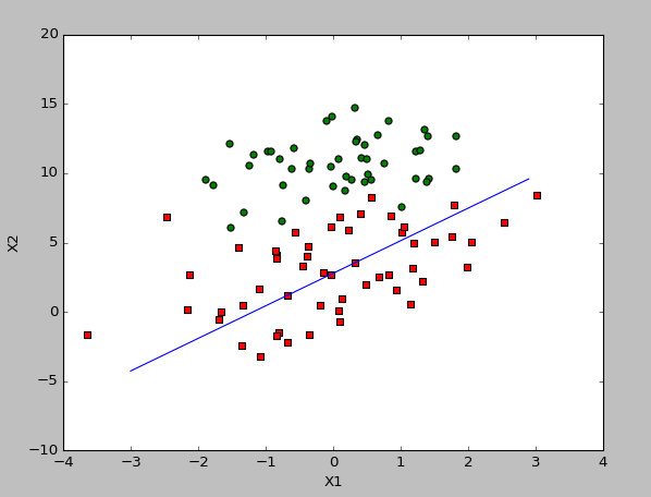
在main.py中调用可以得到下面的决策面
import numpy as np
import logistic as reg
dataArr,labelMat = reg.loadDataSet()
weights = reg.gradAscent(dataArr, labelMat)
weights = weights.getA()
print weights
reg.plotBestFit(weights)
从图中可以看出,基本能正确分出这两类,边界分的较好,只有少数几个点未分出来。
6.5.将梯度上升改为随机梯度上升,在logistic.py中继续添加下面代码
def stocGradAscent0(dataMat, classLabels):
dataMat = np.array(dataMat)
m,n = np.shape(dataMat)
alpha = 0.01
weights = np.ones(n)
for i in xrange(m):
h = sigmoid(sum(dataMat[i]*weights))
error = classLabels[i]-h
weights = weights + alpha*error*dataMat[i]
return weights
那么随机梯度上升和梯度上升有什么不一样?从代码中我们可以看到,h = sigmoid(sum(dataMat[i]*weights))这里dataMat[i]是一个数,不再是一个向量,同样输出h也是一个数,这样算下来,这个代码在数据集上只计算了一样,和上面默认设置的600次相比,计算量大大减少。下面在main.py中调用下,看下效果。
import numpy as np
import logistic as reg
dataArr,labelMat = reg.loadDataSet()
weights = reg.stocGradAscent0(dataArr, labelMat)
print weights
reg.plotBestFit(weights)
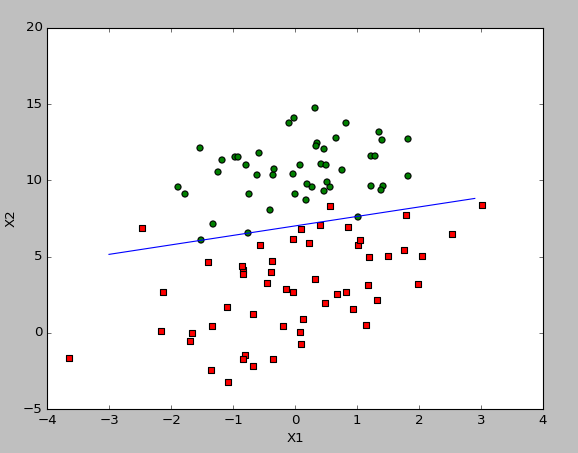
从图中可以看到,效果很一般,有很多都没有分出来,那么是不是随机梯度算法就不适合呢,并不是,导致上面的主要原因是算法并未收敛,下面是改进的算法,使其在整个数据集上的迭代次数增加,并收敛。在logistic.py中继续添加
def stocGradAscent1(dataMat, classLabels, numIter=150):
dataMat = np.array(dataMat)
m,n = np.shape(dataMat)
weights = np.ones(n)
for j in xrange(numIter):
dataIndex = range(m)
for i in xrange(m):
alpha = 4/(1.0+j+i)+0.01
randIndex = int(np.random.uniform(0,len(dataIndex)))
h = sigmoid(sum(dataMat[randIndex]*weights))
error = classLabels[randIndex]-h
weights = weights + alpha*error*dataMat[randIndex]
del(dataIndex[randIndex])
return weights
在main.py中调用,得到如下结果:
import numpy as np
import logistic as reg
dataArr,labelMat = reg.loadDataSet()
weights = reg.stocGradAscent1(dataArr, labelMat)
print weights
reg.plotBestFit(weights)
可以看到改进的随机梯度上升算法和原算法分类基本一样,但计算量更少,且学习率自适应下降,随机选取样本,更有说服力。
7.例子2:从疝气病预测病马的死亡率,数据包括368个样本和38个特征,数据来自2010年1月11日的UCI机器学习数据库。对于样本数据中缺少的数据用0代替,数据处理后保存为两个文件horseColicTestt.txt和horseColicTrining.txt,下面来用logistic回归来分类。在logistic.py中继续添加下面的代码
def classifyVector(inX,weights):
prob = sigmoid(sum(inX*weights))
if prob>0.5:
return 1.0
else:
return 0.0
def colocTest():
frTrain = open('horseColicTraining.txt')
frTest = open('horseColicTest.txt')
trainingSet = []
trainingLabels = []
for line in frTrain.readlines():
currLine = line.strip().split('\t')
lineArr = []
for i in range(21):
lineArr.append(float(currLine[i]))
trainingSet.append(lineArr)
trainingLabels.append(float(currLine[21]))
trainWeights = stocGradAscent1(trainingSet, trainingLabels,500)
errorCount =0.0
numTestVec =0.0
for line in frTest.readlines():
numTestVec +=1.0
currLine = line.strip().split('\t')
lineArr = []
for i in range(21):
lineArr.append(float(currLine[i]))
if int(classifyVector(lineArr,trainWeights)!=int(currLine[21])):
errorCount +=1
errorRate = (float(errorCount)/numTestVec)
print "the error rate of this test is:%f" % errorRate
return errorRate
def multiTest():
numTests = 10
errorSum = 0.0
for k in range(numTests):
errorSum += colocTest()
print "after %d iteration the average error rate is: %f" % (numTests,errorSum/float(numTests))
多次测试,取平均输出如下
the error rate of this test is:0.373134
the error rate of this test is:0.388060
the error rate of this test is:0.432836
the error rate of this test is:0.253731
the error rate of this test is:0.328358
the error rate of this test is:0.417910
the error rate of this test is:0.492537
the error rate of this test is:0.417910
the error rate of this test is:0.268657
the error rate of this test is:0.283582
after 10 iteration the average error rate is: 0.365672
在数据缺失的情况下可以达到36%左右的平均错误率已经很不错了。
所有数据集合及源码,请戳这里