Probabilistic Interpretation on Least Squares

Probabilistic Interpretation on Least Squares

Ethara

Suppose you are asked to make a regression on a training set,

Figure 1

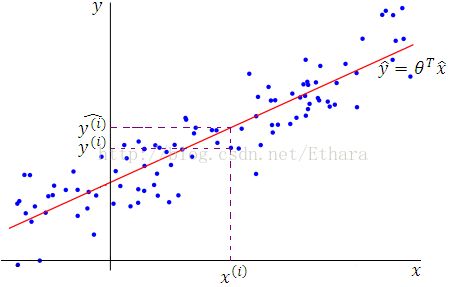
You might want to find a line as in the Figure 1.

Formally, to find an analytical form of this regression line, we need to formalize this problem by,

In this paper, what I want to do is to present two probabilistic interpretations on Least Squares, maximum likelihood (ML) on frequentist statistics and maximum a posteriori (MAP) estimate on Bayesian School, which are two different probabilistic views of the world.

Frequentist Statistic

In the frequentist view of this world, the parameter theta is thought of as being constant-valued but unknown rather than random---it just happens to be unknown---and it’s our job to come up with statistical procedures (such as maximum likelihood) to try to estimate this parameter (as described in Part VII Regularization and model selection of Andrew Ng’s lecture notes on machine learning).

Hence, using ML, we need to choose the parameters according to

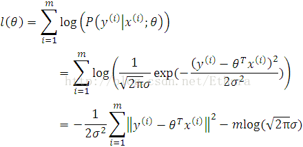
Writing down the log likelihood of the objective function to be maximized,

To formulate

we are convinced that the target variables and the inputs are related via the equation (See Figure 1 to get an intuition),

where epsilon⁽ⁱ⁾ is the ith error term that captures either unmodeled effects or random noise. Furthermore, let us assume that the epsilon⁽ⁱ⁾ are distributed IID (independently and identically distributed) according to a Gaussian distribution with mean zero and some variance sigma².

Writing this assumption as

i.e. the probability density of epsilon⁽ⁱ⁾ is given by

This implies that

i.e. the probability density of y⁽ⁱ⁾| x⁽ⁱ⁾ is given by

Note that we should not condition on theta, since theta is not a random variable in the view of frequentist statistics.

Back into our problem to maximize l(.) (since the principal of ML says that we should choose the parameters so as to make the data as high probability as possible),

Hence, maximizing l(.) gives the same answer as minimizing

which is recognized to be J(.), our original least squares cost function.

Bayesian School

The Bayesian view of the world is an alternative way to approach parameter estimation problems. In this approach, we insist that theta is an unknown random variable with a prior distribution p(.) on it. Practically, a common choice for the prior p(.) is to assume that

Then, given a training set S, we can compute the posterior distribution on the parameters,

Unfortunately, in general, it is computationally very difficult to compute this posterior distribution in closed-form, since it requires taking integrals over the (usually high-dimensional) theta.

One common approximation to this problem, the MAP (maximum a posteriori) estimate for theta is given by

(Compare this with ML).

Likewise, we will prove that the MAP estimate gives the same answer as minimizing some least-squares-like cost function like

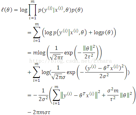
Writing down the log likelihood of MAP,

Therefore, maximizing the above log likelihood gives the same answer as minimizing

Hence,

The proof is completed.

Acknowledgement

This work was inspired by an innovative question raised by C. Huang who is a graduate-to-be of PKU. Some discussions were abstracted from Andrew Ng’s lecture notes on machine learning.

Postscript

May I draw a bold conclusion? Gaussian distribution is the God’s Hallows.