Derivation on Central Limit Theorem

Derivation on Central Limit Theorem

Ethara

Here comes something really spooky.

Suppose a random signal is created by generating a bunch of random numbers in between 0 and 1 and joining them by straight lines, then we can have its cartoon shown in Figure 1 (a). As we take convolutions on the random signal with itself iteratively, something spooky really happens that we get a bell-shaped curve just after three times convolutions.

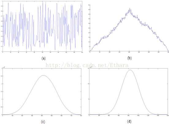
Figure 1. (a) shows the initial random signal. It turns to (b) after one convolution. It turns to (c) after two convolutions. It turns to (d) after three convolutions.

As a matter of fact, after taking infinite many times of convolutions, we shall get a Gaussian distribution, as shown in Figure 2.

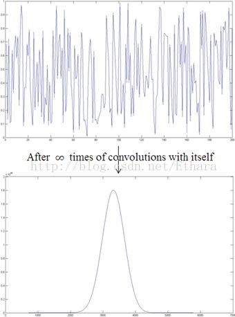
Figure 2

Problem is, how could this spookiness possibly happen?

Central Limit Theorem

The answer lies in Central Limit Theorem (CLT) manipulating this entire magical and charming math game,

Given a sequence of random variables which are iid (independent identically distributed), {X₁, …, X_n}, and,

for any real number x,

Digression

What I want to do in this paper is to derive CLT. Before the derivation, we need to come to a digression on convolution.

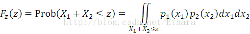
Suppose X₁ and X₂ are independent random variables with distributions p₁(x₁) and p₂(x₂), then what is the distribution of Z = X₁ + X₂?

For any value of z,

With change of variables, u = x₁, x₁ + x₂ = v,

Thus, the distribution of Z = X₁+ X₂ is,

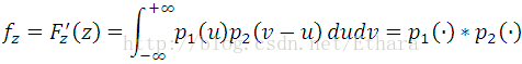
More generally, the distribution of X₁ + … + X_n is p₁*…*p_n.

Derivation on CLT

Now let us return to the derivation on CLT.

With normalization to variables, we can simply take the following assumption,

Let S_n denote the sum of n items, i.e. S_n = X₁+ … + X_n, then the mean of S_n is 0 and the standard deviation is sqrt(n).

After further normalization to S_n,

then, the mean of Y_n is 0 and the standard deviation is 1.

Let p_n(x) denote the distribution of Y_n, we will see,

Since X₁, …, X_n are iid, we have, p(x) = p₁(x₁) = … = p_n(x_n).

Therefore, the distribution of X₁ + …+ X_n is,

Let y_i = x_i / sqrt(n), then,

Thus, the distribution of Y_n is,

Now take Fourier transform of p_n(x) in order to turn convolution into multiplication for an easier derivation,

where

Take inverse Fourier transform,

Therefore, in conclusion,

Now the spookiness can be easily explained by CLT.

CLT indicates that, no matter what distribution X_i’s conform to, as long as {X_i, i = 1, …, n} are iid and n is sufficiently large, we come to the approximation that,

i.e.,

DeMoivre-Laplace Theorem

In particular, when X_i’s conform to B(1, p), we will see DeMoivre-Laplace Theorem derived from CLT,

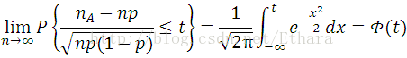
where n_A is the number of times for which Event A happens in a n-time Bernoulli experiment.

Example

Suppose you are attending a CET-4, 6 exam today, there are 85 choice questions. Each has four choices with only one to be correct. Those who want to pass the exam must give right answers to more than 51 questions. Question is, what is the probability of one passing the exam purely by luck?

Solution:

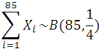
Define random variables, (i = 1, …, 85)

are iid. Further,

Using DeMoivre-Laplace Theorem yields,

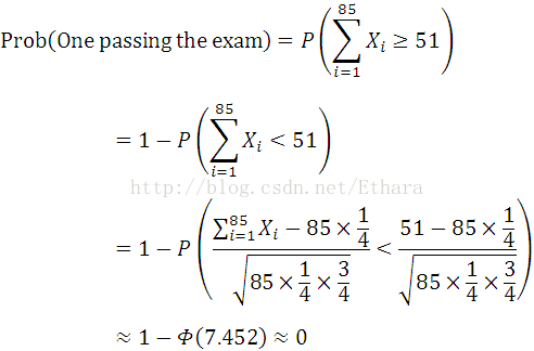
This indicates that, improvement on English ability is the only way to pass a CET-4,6 exam.

Acknowledgement

The whole discussion above benefits highly from Professor Osgood’s course on Fourier transform and its application of Stanford University. The cartoons are provided by Junjie WANG, who is an undergraduate in BJTU.