R Graphics Basics: Plot area, mar (margins),oma (outer margin area),mfrow, mfcol (multiple figures)
http://research.stowers-institute.org/efg/R/Graphics/Basics/mar-oma/index.htm
Purpose
This technote explains how to use certain R graphics parameters that deal with margins, namely mar and oma. The usage of these parameters is explained for plotting a single figure, and for plotting multiple figures.
Background
R is such a graphics-rich analysis language, yet ironically the description of many of its graphics features are not explained visually. R's graphical parameters (see ?par) are a bit overwhelming and the alphabetical order of the dozens and dozens of parameters -- there are more than 70 -- in the online documentation doesn't help beginners discern groups and relationships among these parameters very easily. [Too many software developers ignore the Psychological Review paper, "The Magical Number Seven, Plus or Minus Two: Some Limits on Our Capacity for Processing Information," when they develop software and documentation.]
This Technote attempts to explain several of the graphics parameters, par, and in particular the ones that deal with margins. The mar parameter defines the margins for a figure, and the oma parameter defines the "outer margin area" around a figure or figures. The usage of mar and oma is shown when plotting a single figure, and when plotting multiple figures, using the mfrow or mfcol parameters.
Software Requirements
Tested in R 2.1.1
Step-by-Step Procedure
Execute the R code described below to better understand this example. You can download the code from the following link, or just source it from here by copying and pasting this statement into R:
source("http://research.stowers-institute.org/efg/R/Graphics/Basics/mar-oma/mar-oma.R")
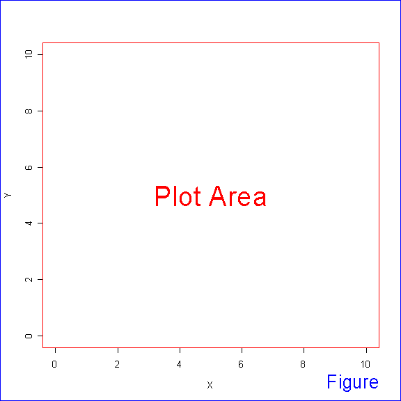
1. The R Plot Area. The plot statement below is typical of a simple "XY" plot R. In this example, the line is suppressed but the X and Y axes can be seen. In Figure 1 the "plot area" is inside the red box, and the perimeter of the figure is shown in a blue box.
Run the Figure1() function to see this figure, which could be created with the following R statements:
|
plot(0:10, 0:10, type="n", xlab="X", ylab="Y") text(5,5, ID, col="red", cex=size1) box("plot", col="red") mtext("Figure", SOUTH<-1, line=3, adj=1.0, box("figure", col="blue") |
Figure 1. The R Plot Area
The area between the red box and the blue box is known as the "margin" area, and is controlled by the R mar parameter. You can view the value of mar at any time from the R command line:
> par()$mar
[1] 5.1 4.1 4.1 2.1
These values will be described in more detail in the next step, but you can see the margin at the bottom (the "south" side on a map) is about 5 lines and the margin at the left (the "west" side) is about 4 lines. Likewise, the margin at the top (the "north" side) is also about four lines, while the margin at the right (the "east" side) is only 2 lines. The size of the margin areas reflects typical needs for labels for the axes, as well as a title at the top of the plot.
You can set the mar parameter to other values using the par function:
> par(mar=c(4, 4, 2, 0.5))
Note that even though the margin is measured in "lines", the values need not be integers.
There is no "outer margin area" in this simple example, which is typical of many R plots.
The Figure1 function actually makes use of a GenericFigure function which is also used in subsequent examples. Convince yourself that this code is equivalent to the code shown above.
|
GenericFigure <- function(ID, size1, size2) # Figure 1. Default R Plot Area / Figure Area |
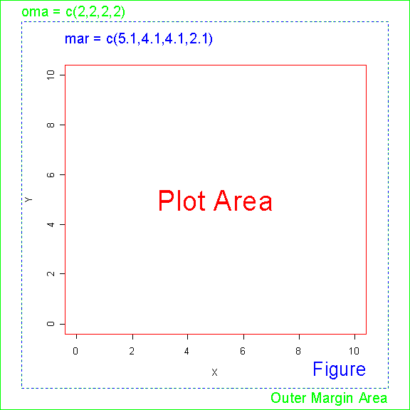
2. The Outer Margin Area. Let's extend the example above to include an "outer margin area," or oma. Display Figure 2A, shown below, by running the function Figure2A().
Figure 2A. The R Plot Area with Outer Margin Area
(Note: the plot area is in red,
the figure's margin area text and outline are in blue,
and the text and outline of the outer margin area are in green)
These R statements provide a 2-line outer margin area on all four sides of the original Figure 1.
|
par(oma=c(2,2,2,2)) GenericFigure("Plot Area", 3,2) # "figure" box and "inner" margin box same for single figure plot mtext("Outer Margin Area", SOUTH<-1, line=0.4, adj=1.0, cex=1.5, |
The values for the current margin area, mar, and outer margin area, oma, are shown in Figure 2A. How was this added to the figure?
|
Margins <- capture.output( par()$mar ) |
We saw above that the margin values can be easily interrogated:
> par()$mar
[1] 5.1 4.1 4.1 2.1
After using R's capture.output statement, we can manipulate the output line shown in black. R's substr function is used to drop the "[1]" from the output string. gsub is used to replace blanks with commas, and paste is used to form the final string used in the mtext display of the margin values. A similar construct displays the oma values. But where did the assignments, NORTH<-3 and SOUTH<-1, shown above, originate?
I find R's use of arbitrary constants for "sides" (like "1" for "bottom") a bit puzzling since the use of mnemonic constants for such values has been an established software engineering practice for at least two decades now. (See Code Complete 2, Section 12.7, "Named Constants.") I don't have the rhetorical skills necessary to convince the R core team to change their ways and define such constants for all R users (I think they claim they don't want to have "namespace pollution"), but I choose to use mnemonic constants in my code. For example, I use SOUTH<-1, WEST<-2, NORTH<-3, and EAST<-4, since most are familiar with map directions, and this puts all four values on a common basis.
The four sides of the figure's margin area, and outer margin area, are annotated below in Figure 2B with the directional mnemonics.
|
Figure2A() # Text: one string per mtext call # Text: vector of strings in mtext call |
Figure 2B. Margin Area and Outer Margin Area "Directions":
South, West, North, East
One especially good use of the outer margin area is to put a time stamp at the bottom of every graphic (in case you're a clock watcher, anal retentive, or work in quality control, or a regulated industry -- I've had all four problems):
|
par(oma=c(1.5,0,0,0)) # 1.5 line2 at the bottom shortname <- "Figure1" # or maybe a filename |
Figure 2C. Time Stamp Added in Outer Margin Area
3. Multiple Figures. R provides several ways to plot more than one figure on a graphics device. The simplest is to use the par function and define the "multiple figures by column" parameter, mfcol, or the multiple figures by row, mfrow. The first example here shows mfrow, while the second shows mfcol.
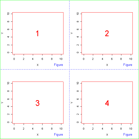
Here's is the code to create the Figure3A example (shown below), or simply run Figure3A() in R to see it on your screen..
|
MultipleFigures <- function() GenericFigure("2", 3,1) GenericFigure("3", 3,1) GenericFigure("4", 3,1) # Figure 3A. Using Multiple Figures. MultipleFigures() |
The numbers in the mfrow=c(2,2)definition tell how many rows and columns of figures to be plotted on the graphics device.
c(4,3) would mean 4 rows of 3 columns of figures for a total of 12 figures on the graphics device. mfrow means to plot the figures in row 1 from left-to-right, followed by row 2 from left-to-right, etc. mfcol means to plot the figures in column 1 from top-to-bottom, followed by the figures in column 2 from top-to-bottom, etc.
With the code shown above, the figures are plotted from left-to-right in two rows in Figure 2B. The normal "R" default values for mar=c(5.1,4.1,4.1,2.1)and oma=c(0,0,0,0) are set explicitly above for emphasis.
Figure 3A. Multiple Figures by Row (mfrow) With No Outer Margin Area
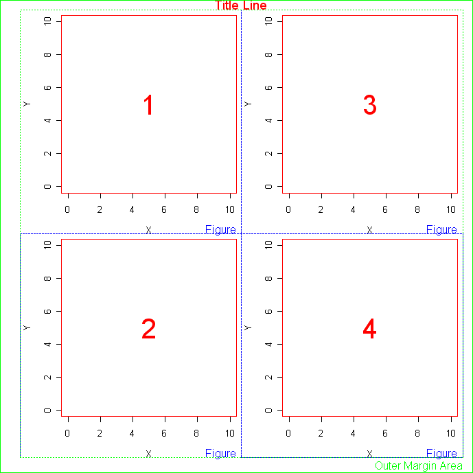
Note the default margins specified by mar can result in excessive white space between the plots. Let's modify Figure 3A to have less white space around the plots, and a slim outer margin area around the page:
|
# Figure 3B. Using Multiple Figures with outer margin area MultipleFigures() mtext("Outer Margin Area", box("outer", lty="solid", col="green") |
The mar=c(4,4,0.5,0.5) definition gives 4 lines of margin space at the bottom and left for the X and Y axes, and little space at the top and right -- if you had a title you would want to reserve more space at the top. The oma=c(1.5,2,1,1) definition reserves 1.5 lines at the bottom for the outer margin area, which would be useful for the time stamp example shown above. 2 lines were reserved at the top for the "Title Line", with one line reserved on the left and right sides.
Figure 3B. Multiple Figures by Row (mfcol) With Slim Outer Margin Area


