Bézier Triangles and N-Patches
The advantage of using curved surfaces is at least fourfold:
- they have a more compact representation than a set of polygons,
. - they provide scalable geometric primitives,
. - they provide smoother and more continuous primitives than planar polygons,
. - animation and collision detection may become simpler and faster.
.
There are a number of advantages of a compact curve representation for real-time rendering.
- There is a savings in memory for model storage (and so some gain in memory cache efficiency). This is especially useful for game consoles, which typically have little memory compared to a PC.
. - Transforming curved surfaces generally involves fewer matrix multiplications than transforming a mesh representing the surface.
. - If the graphics hardware can accept such curved surface descriptions directly, the amount of data the host CPU has to send to the graphics hardware is usually much less than sending a polygon mesh.
.
This article starts with a brief description of Bézier triangles. Bézier triangles form the basis for N-patches, which are discussed in more detail in the rest of the article.
Bézier Triangles
Even though the triangle often is considered a simpler geometric primitive than the rectangle, this is not the case when it comes to Bézier surfaces: Bézier triangles are not as straightforward as Bézier patches. However, because Bézier triangles are used in forming N-patches, we first discuss these.
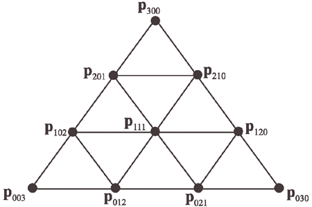
The control points are located in a triangular grid, as shown in Figure 1.
Figure 1. The control points of a Bézier triangle with degree three (cubic).
The degree of the Bézier triangle is n, and this implies that there are n+1 control points per side. These control points are denoted p0i,j,k and sometimes abbreviated to pi,j,k. Note that i+j+k=n, and i,j,k >= 0 for all control points. Thus, the total number of control points is
It should come as no surprise that Bézier triangles also are based on repeated interpolation. However, due to the triangular shape of the domain, barycentric coordinates must be used for the interpolation. Recall that a point within a triangle Δp0p1p2, can be described as
p(u,v) = p0 + u(p1-p0) + v(p2-p0) = (1-u-v)p0 + up1 + vp2,
where (u,v) are the barycentric coordinates. For points inside the triangle the following must hold: u>=0, v>=0, and 1-u+v>=0 (alternately, u+v<=1). Based on this, the de Casteljau algorithm for Bézier triangles is:
de Casteljau [triangles]:
The final point on the Bézier triangle at (u,v) is pn000(u,v). The Bézier triangle in Bernstein form is:
Bernstein [triangles]:
The Bernstein polynomials now depend on both u and v, and are therefore computed differently, as shown below:
When any of the following is true: i,j,k<0 and i,j,k>n, the Bernstein polynomial is set to zero; Bnijk(u,v)=0. The partial derivatives are [1]:
Derivatives [triangles]:
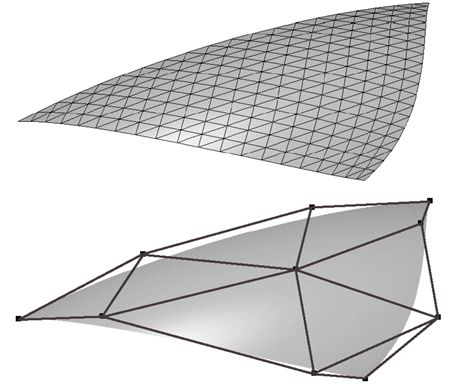
Some unsurprising properties of Bézier triangles are that they interpolate (pass through) the three corner control points, and that each boundary is a Bézier curve described by the control points on that boundary. Also, the surfaces lies in the convex hull of the control points. Finally, rotating the control points and then generating points on the Bézier triangle is the same as generating points on the Bézier triangle and then rotating these. A Bézier triangle is shown in Figure 2.
Figure 2. Top: wireframe of a Bézier triangle. Bottom: Shaded surface together with control points.
Next, we will discuss a direct application of Bézier triangles.
N-Patches
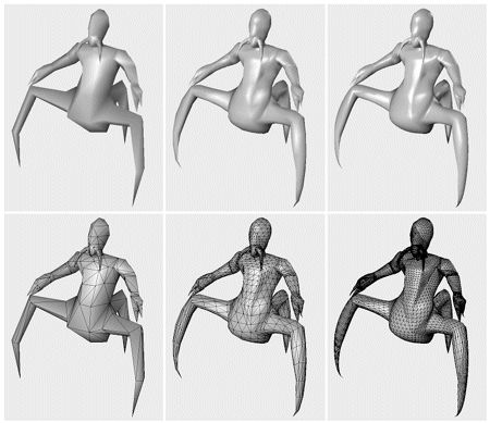
Given an input triangle mesh with normals at each vertex, the goal of the N-patches scheme by Vlachos et al. [2] is to construct a better looking surface on a triangle basis. The term "N-patches" is short for "Normal-Patches," and these patches are also called PN triangles. This scheme attempts to improve the triangle mesh's shading and silhouette by creating a curved surface to replace each triangle. Hardware is able to make each surface on the fly because the tessellation is generated from each triangle's points and normals, with no neighbor information needed. API changes are minimal; all that is needed is a flag telling whether to generate N-patches, and a level of tessellation. See Figure 3 for an example. The algorithm presented here builds upon work by van Overveld and Wyvill [3].
Figure 3. The columns show different levels of detail of the same model. The original triangle data, consisting of 414 triangles, is shown on the left. The middle model has 3,726 triangles, while the right has 20,286 triangles, all generated with the presented algorithm. Note how the silhouette and the shading improves. The bottom rows show the models in wireframe, which reveals that each original triangle generates the same amount of subtriangles. (Model courtesy of id Software. Image from ATI Technologies Inc. demo.)
Assume we have a triangle with vertices p300, p030, and p003 with normals n200, n020, and n002. The basic idea is to use this information to create a cubic Bézier triangle for each original triangle, and generate as many triangles as we wish from the Bézier triangle.
To shorten notation, w = 1-u-v will be used. A cubic Bézier triangle (see Figure 1) is given by:
To ensure C0 continuity at the borders between two N-patch triangles, the control points on the edge can be determined from the corner control points and the normals at the respective control point (assuming that normals are shared between adjacent triangles). Also, to get reasonable behavior of the surface at the control points, the normals there should be normals of the surface in the equation above. Therefore, the following strategy is adopted to compute the six different control points for the borders. Say that we want to compute p210 using the control points p300, p030, and the normal n200 at p300. Simply take the point 2/3 p300 + 1/3 p030 and project it in the direction of the normal, n200, onto the tangent plane defined by p300 and n200 [2][5][1]. See Figure 4.
Figure 4. How the Bézier point p210 is computed using the normal n200 at p300, and the two corner points p300 and p030.
Assuming normalized normals, the point p210 is computed as:
The other border control points can be computed similarly, so it only remains to compute the interior control point, p111. This is done as shown in the equation that follows, and this choice follows a quadratic polynomial [5][1]:
Instead of using the previous Bézier triangle derivatives equation to compute the two tangents on the surface, and subsequently the normal, Vlachos et al. [2] choose to interpolate the normal using a quadratic scheme as shown below:
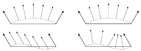
This can be thought of as a Bézier triangle of degree two, where the control points are six different normals. In the equation above, the choice of the degree, i.e., quadratic, is quite natural since the derivatives are of one degree lower than the actual Bézier triangle, and because linear interpolation of the normals cannot describe an inflection. See Figure 5.
Figure 5. This figure illustrates why quadratic interpolation of normals is needed, and why linear interpolation is not sufficient. The left column shows what happens when linear interpolation of normals are used. This works fine when the normals describe a convex surface (top), but breaks down when the surface has an inflection (bottom). The right column illustrates quadratic interpolation. (Illustration after van Overveld and Wyvill [6].)
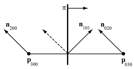
To be able to use the previous equation, the normal control points n110, n101, and n011, need to be computed. One intuitive, but flawed, solution is to use the average of n200 and n020 (normals at the vertices of the original triangle) to compute n110. However, when n200=n020, then the problem shown at the lower left in Figure 5 will once again be encountered. Instead, n110 is constructed by taking the average of n200 and n020. Then this normal is reflected in the plane π, which is shown in Figure 6. This plane has a normal parallel to the difference between the endpoints; p300 and n030. The plane π is passing through the origin since direction vectors are reflected, and these are independent on the position on the plane. Also, note that each normal should be normalized.
Figure 6. Construction of n010 for N-patches. The dashed normal is the average of n200 and n020, and n010 is this normal reflected in the plane π. The plane π has a normal that is parallel to p030-p300.
Mathematically, the unnormalized version of n110 is expressed as [2]:
van Overveld and Wyvill originally used a factor 3/2 instead of the 2 in the equation above. Which value is best is hard to judge from looking at images, but using 2 gives the nice interpretation of a true reflection in the plane. Lee and Jen analyze artifacts involved in normal interpolation, and suggest solutions [4].
At this point, all Bézier points of the cubic Bézier triangle and all the normal vectors for quadratic interpolation have been computed. It only remains to create triangles on the Bézier triangle so these can be rendered. Advantages of this approach are that the surface gets a better silhouette and shape relatively cheaply, and that only minor modifications must be made to existing code to make this work. All that is needed is that tessellation should be done (instead of rendering as usual), down to some Level of Detail (LOD). A hardware implementation is pretty straightforward.
One way to specify LODs is the following. The original triangle data is LOD 0. Then the LOD number increases with the number of newly introduced vertices on a triangle edge. So LOD 1 introduces one new vertex per edge, and so creates four subtriangles on the Bézier triangle, and LOD 2 introduces two new vertices per edge, generating nine triangles. In general, LOD n generates (n+1)² triangles. To prevent cracking between Bézier triangles, each triangle in the mesh must be tessellated with the same LOD. This is a big disadvantage since a tiny triangle will be tessellated as much as a large triangle. Adaptive tessellation and fractional tessellation are possible, but not yet supported. Creases are hard to control, and often one needs to insert extra triangles near the desired crease. The continuity between Bézier triangles is only C0, but still it looks acceptable in many cases. This is mainly because the normals are continuous across triangles, so that a set of N-patches mimic a G1 surface. Note that to get good looking texturing, C1 continuity is required across borders between triangles (or patches). Also worth knowing is that cracks will appear if two adjacent triangles do not share the same normals.
API and Hardware Support
N-patches are supported by the DirectX 8 API and through extensions in OpenGL. Version 8.0 of DirectX has support for the interpolation of normals, but only with linear interpolation. Version 8.1 also allows quadratic interpolation of normals. There is a performance cost in normal interpolation; quadratic interpolation is more expensive than linear. Besides the standard N-patch interpolation (cubic Bézier triangles), version 8.1 also allows linear interpolation of vertex positions. This means that a triangle is tessellated with many smaller coplanar triangles with interpolated normals across each. ATI accelerates N-patches in hardware, which they call TRUFORM, beginning with their 8000 series of chips. N-patches are also used in the displacement mapping primitive proposed by Matrox.
Acknowledgements
We would like to thank Alex Vlachos for his help consulting on parts of this article.
References
[1] Farin, Gerald, Curves and Surfaces for Computer Aided Geometric Design--A Practical Guide, Fourth Edition (First Edition, 1988), Academic Press Inc., 1996.
[2] Vlachos, Alex, Jörg Peters, Chas Boyd, and Jason L. Mitchell, "Curved PN Triangles," ACM Symposium on Interactive 3D Graphics 2001, pp. 159-166, 2001. http://alex.vlachos.com/graphics/CurvedPNTriangles.pdf
[3] van Overveld, C.V.A.M., and B. Wyvill, "An Algorithm for Polygon Subdivision Based on Vertex Normals," Computer Graphics International '97, pp. 3-12, June 1997.
[4] Leed, Yuan-Chung, and Chein-Wei Jen, "Improved Quadratic Normal Vector Interpolation for Realistic Shading," The Visual Computer, vol. 17, no. 6, pp. 337-352, 2001.
[5] Farin, Gerald, "Triangular Bernstein-Bézier Patches," Computer Aided Geometric Design, vol. 3, no. 2, pp. 83-127, 1986.
[6] van Overveld, C.V.A.M., and B. Wyvill, "Phong Normal Interpolation Revisited," ACM Transaction on Graphics, vol. 16, no. 4, pp. 379-419, October 1997.
from : http://www.gamasutra.com/features/20020715/mollerhaines_01.htm
http://www.gamasutra.com/features/20020715/mollerhaines_02.htm
