深度学习图像分类（一）——AlexNet论文理解

0. 写作目的

好记性不如烂笔头。

1. 论文理解

1.1 ReLU 激活函数的使用

Rectified Linear Units(ReLU)

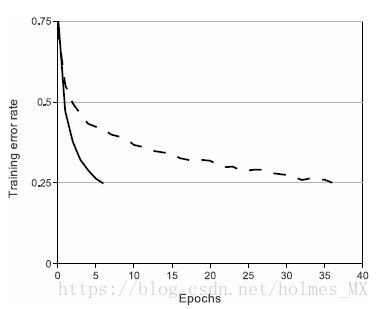
使用ReLU比使用tanh（或者sigmoid）激活函数收敛速度更快。下图来自AlexNet论文中给出的在CIFAR-10上的测试效果。可以看出ReLU收敛速度更快。

1.2 多GPU训练

只在特殊层进行GPU数据之间的交流。

例如：第3卷积层的Feature map全部来自于第2卷积层(即来自不同GPU)，但第4卷积层的Feature map只来自同一GPU的feature map. 

相比只使用一个GPU进行训练，多个GPU信息交互，可以提高精度： 1.7%(top-1)。

1.3 Local Response Normalization (LRN)

文章说： LRN可以增加 泛化能力。

由于后继的分类网络说，LRN效果并不是很好，所以后继的网络都未加入该层。因此这里简单介绍一下。

LRN即对于一个feature map（N个channel）的其中一个channel，将该层前后各n个channel对应位置的数值，然后进行归一化。具体可以看下面的公式：

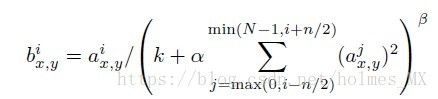
其中， (x, y)是channel中的位置， i是第i个channel，n 是相邻的“前后”n 个channel数，N是该feature map总的channel数目（即边界channel的处理），实验中k = 2, n = 5, aerfa = 1e-4, belta = 0.75。参数是通过交叉验证得到的。

LRN的使用位置：使用在特征层的ReLU激活函数后。

文中给出的性能提升：LRN可以看做是一种“亮度的正则化（brightness normaliztion）”。因为作者并没有减去均值。

LRN降低1.4%的error rates （TOP-1）， 在CIFAR-10验证的效果是降低2% test error rate。

1.4 Overlapping Pooling

采用重叠池化。

采用的s = 2 (stride), z = 3, 可以降低0.4%（TOP-1）error rates与 s = 2, z = 2(正常的池化，即无重叠池化)。

作者发现：使用Overlapping Pooling 可以轻微地减少过拟合。

2. AlexNet网络

网络为：   5 conv + 3 fully-connect（输入层不算）

上图中： 150528 = 224 * 224 * 3

从上图看出： GPU进行交叉的层是： 第3层、第6层（fc-1）、第7层（fc-2）、第8层(softmax)。

使用LRN层的是： 第1卷积层和第2卷积层， ReLU之后。

MaxPooling层：在第1卷积层、第2卷积层和第5卷积层后。

ReLU应用在每个卷积层和全连接层后（除了最后一层）。

实际的网络为：给出基于tensorflow的AlexNet（未使用多个GPU）

并附上AlexNet的代码

import os
import keras
import tensorflow as tf

def print_Layer(layer):
    print(layer.op.name, ' ', layer.get_shape().as_list())
tf.reset_default_graph()
    
def AlexNet():
    input = tf.keras.Input( shape=(224, 224, 3), name='alexNet_input' )
    print_Layer(input)
    
    ## conv1
    conv1 = tf.keras.layers.Conv2D( filters=96, kernel_size=(11,11), strides=(4,4), padding='same', activation=tf.nn.relu, name='conv1')(input)
    print_Layer(conv1)
    x = tf.nn.local_response_normalization( conv1, depth_radius=5, bias=1, alpha=1, beta=0.5, name='LRN-1')
    print_Layer(x)
    
    ## MaxPool
    maxpool1 = tf.keras.layers.MaxPooling2D( pool_size=(3, 3), strides=(2, 2), padding='valid', name='MaxPool1' )(x)
    print_Layer(maxpool1)
    
    ## conv2
    conv2 = tf.keras.layers.Conv2D( filters=256, kernel_size=(5,5), strides=(1,1), padding='same', activation=tf.nn.relu, name='conv2' )(maxpool1)
    print_Layer(conv2)
    x = tf.nn.local_response_normalization( conv2, depth_radius=5, bias=1, alpha=1, beta=0.5, name='LRN-2')
    print_Layer(x)
    
    ## MaxPool
    maxpool2 = tf.keras.layers.MaxPooling2D( pool_size=(3, 3), strides=(2, 2), padding='valid', name='MaxPool2' )(x)
    print_Layer(maxpool2)
    
    ## conv3
    conv3 = tf.keras.layers.Conv2D( filters=384, kernel_size=(3,3), strides=(1,1), padding='same', activation=tf.nn.relu, name='conv3')(maxpool2)
    print_Layer(conv3)
    
    ## conv4
    conv4 = tf.keras.layers.Conv2D( filters=384, kernel_size=(3,3), strides=(1,1), padding='same', activation=tf.nn.relu, name='conv4')(conv3)
    print_Layer(conv4)
    
    ## conv5
    conv5 = tf.keras.layers.Conv2D( filters=256, kernel_size=(3,3), strides=(1,1), padding='same', activation=tf.nn.relu, name='conv5' )(conv4)
    print_Layer(conv5)
    
    ## MaxPool
    maxpool3 = tf.keras.layers.MaxPooling2D( pool_size=(3, 3), strides=(2, 2), padding='valid', name='MaxPool3' )(conv5)
    print_Layer(maxpool3)
    
    ## flatten
    flat = tf.keras.layers.Flatten(name='Flat')(maxpool3)
    print_Layer(flat)
    
    ## fc-1
    fc1 = tf.keras.layers.Dense( units = 4096, activation=tf.nn.relu, name='fc1' )(flat)
    print_Layer(fc1)
    
    ##fc-2
    fc2 = tf.keras.layers.Dense( units = 4096, activation=tf.nn.relu, name='fc2' )(fc1)
    print_Layer(fc2)
    
    ## output
    predict = tf.keras.layers.Dense( units = 1000, activation=tf.nn.softmax, name='predict' )(fc2)
    print_Layer(predict)
    
    return predict

AlexNet()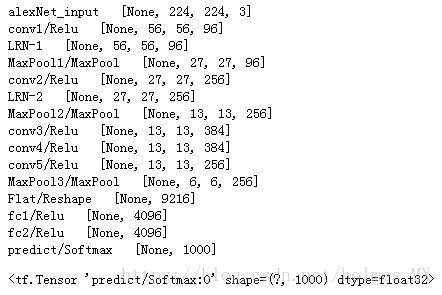

3. 训练的细节

3.1 降低过拟合

（1） 数据增强 Data Augmentation

第一种是：图像变换和水平镜像。

训练时： 从256*256的图像中，先进行，crop 224 * 224的图像。

测试时： 从图像中，crop 224*224的图像（10个， (four corner + center) * 2）镜像的结果，将10个结果取softmax输出结果的均值。

第二种是：改变RGBchannel的强度。

对每个训练图像，先使用PCA（主成分分析）求出特征值和特征向量（以RGB为特征，将图像看成一维的，然后计算），然后在特征值上乘以一个随机数，再将修改后的特征值与特征向量相乘，得到RGB channel强度变换后的值。随机数的产生：均值为0，方差为0.1的高斯随机数。

 

（2） Dropout

结合多个模型的预测结果是降低test errors的好方法，但是太耗时间，因此使用Dropout来降低过拟合。

Dropout可解释：每次训练时都是不同的网络（由于Drop的点不一样）； 降低不同神经元之间的联系。

训练时，在两个全连接层使用Droptout( 0.5 )。测试时，计算所有神经元，但是结果*0.5.

3.2 训练参数

SGD + batch_size(128)  +  momentum (0.9) + weight decay (0.0005)

发现weight decay 对模型的学习很重要。不仅仅是正则化，也降低了test errors.

权重更新公式：

权重的初始化： 均值为0的 方差为0.01的高斯分布。

bias: 第2,4，5卷积层和全连接层初值为1，其他层为0。

当val loss不再下降时，将学习率除以10. 

学习起始值为0.01，训练过程中修改了3次。

大概训练了90个epoch。

There may be some mistakes in this blog. So, any suggestions and comments are welcome!

[Reference]

AlexNet论文：http://papers.nips.cc/paper/4824-imagenet-classification-with-deep-convolutional-neural-networks.pdf