caffe学习--参数调整
- 调整各参数
- 激活函数
- lr
- 修改cifar10中的lr-policy
- 调整lr大小
- dropout
- dropout类型
- 缺点
- 在cifar实例中加入dropout
- batch normalization
- cifar10中的BatchNorm
- data augmentation
- 常见方法
调整各参数
这里用cifar10数据集为例
激活函数
Sigmoid、ReLU、TanH、Absolute Value、Power、BNLL
看一下cifar10中用的是什么激活函数
cifar10_quick.prototxt

还有一种更直观的方法是,我们将训练网络“画”出来
回到caffe的根目录
cd python
python draw_net.py ../examples/cifar10/cifar10_quick.prototxt cifar10.png
因此我们可以清楚的看到这里面三次用到ReLU激活函数
现在我们尝试改一下激活函数,以下是caffe中六种激活函数
layer {
  name: "relu1"
  type: "ReLU"
  bottom: "pool1"
  top: "pool1"
}
layer {
name: "encode1neuron"
bottom: "encode1"
top: "encode1neuron"
type: "Sigmoid"
} layer {
name: "layer"
bottom: "in"
top: "out"
type: "TanH"
} layer {
name: "layer"
bottom: "in"
top: "out"
type: "AbsVal"
} layer {
name: "layer"
bottom: "in"
top: "out"
type: "Power"
power_param {
power: 2
scale: 1
shift: 0
}
} layer {
name: "layer"
bottom: "in"
top: "out"
type: “BNLL”
} 我们来看一下cifar10_quick_train_test.prototxt 的网络图

修改之前:
./build/tools/caffe test \
-model examples/cifar10_quick_train_test.prototxt \
-weights examples/cifar10/cifar10_quick_iter_4000.caffemodel
我们把cifar10里的 cifar10_quick_train_test.prototxt 里的激活函数改成Sigmoid试试
name: "CIFAR10_quick"
layer {
  name: "cifar"
  type: "Data"
  top: "data"
  top: "label"
  include {
    phase: TRAIN
  }
  transform_param {
    mean_file: "examples/cifar10/mean.binaryproto"
  }
  data_param {
    source: "examples/cifar10/cifar10_train_lmdb"
    batch_size: 100
    backend: LMDB
  }
}
layer {
  name: "cifar"
  type: "Data"
  top: "data"
  top: "label"
  include {
    phase: TEST
  }
  transform_param {
    mean_file: "examples/cifar10/mean.binaryproto"
  }
  data_param {
    source: "examples/cifar10/cifar10_test_lmdb"
    batch_size: 100
    backend: LMDB
  }
}
layer {
  name: "conv1"
  type: "Convolution"
  bottom: "data"
  top: "conv1"
  param {
    lr_mult: 1
  }
  param {
    lr_mult: 2
  }
  convolution_param {
    num_output: 32
    pad: 2
    kernel_size: 5
    stride: 1
    weight_filler {
      type: "gaussian"
      std: 0.0001
    }
    bias_filler {
      type: "constant"
    }
  }
}
layer {
  name: "pool1"
  type: "Pooling"
  bottom: "conv1"
  top: "pool1"
  pooling_param {
    pool: MAX
    kernel_size: 3
    stride: 2
  }
}
layer {                 //sigmoid1
  name: "sigmoid1"
  type: "Sigmoid"
  bottom: "pool1"
  top: "pool1"
}
layer {
  name: "conv2"
  type: "Convolution"
  bottom: "pool1"
  top: "conv2"
  param {
    lr_mult: 1
  }
  param {
    lr_mult: 2
  }
  convolution_param {
    num_output: 32
    pad: 2
    kernel_size: 5
    stride: 1
    weight_filler {
      type: "gaussian"
      std: 0.01
    }
    bias_filler {
      type: "constant"
    }
  }
}
layer {                 //sigmoid2
  name: "sigmoid2"
  type: "Sigmoid"
  bottom: "conv2"
  top: "conv2"
}
layer {
  name: "pool2"
  type: "Pooling"
  bottom: "conv2"
  top: "pool2"
  pooling_param {
    pool: AVE
    kernel_size: 3
    stride: 2
  }
}
layer {
  name: "conv3"
  type: "Convolution"
  bottom: "pool2"
  top: "conv3"
  param {
    lr_mult: 1
  }
  param {
    lr_mult: 2
  }
  convolution_param {
    num_output: 64
    pad: 2
    kernel_size: 5
    stride: 1
    weight_filler {
      type: "gaussian"
      std: 0.01
    }
    bias_filler {
      type: "constant"
    }
  }
}
layer {                 //sigmoid3
  name: "sigmoid3"
  type: "Sigmoid"
  bottom: "conv3"
  top: "conv3"
}
layer {
  name: "pool3"
  type: "Pooling"
  bottom: "conv3"
  top: "pool3"
  pooling_param {
    pool: AVE
    kernel_size: 3
    stride: 2
  }
}
layer {
  name: "ip1"
  type: "InnerProduct"
  bottom: "pool3"
  top: "ip1"
  param {
    lr_mult: 1
  }
  param {
    lr_mult: 2
  }
  inner_product_param {
    num_output: 64
    weight_filler {
      type: "gaussian"
      std: 0.1
    }
    bias_filler {
      type: "constant"
    }
  }
}
layer {
  name: "ip2"
  type: "InnerProduct"
  bottom: "ip1"
  top: "ip2"
  param {
    lr_mult: 1
  }
  param {
    lr_mult: 2
  }
  inner_product_param {
    num_output: 10
    weight_filler {
      type: "gaussian"
      std: 0.1
    }
    bias_filler {
      type: "constant"
    }
  }
}
layer {
  name: "accuracy"
  type: "Accuracy"
  bottom: "ip2"
  bottom: "label"
  top: "accuracy"
  include {
    phase: TEST
  }
}
layer {
  name: "loss"
  type: "SoftmaxWithLoss"
  bottom: "ip2"
  bottom: "label"
  top: "loss"
}
可以看出来三个绿色的激活函数都被改成了sigmoid
我们先来测试一下:
./build/tools/caffe test \
-model examples/cifar10_quick_train_test.prototxt \
-weights examples/cifar10/cifar10_quick_iter_4000.caffemodel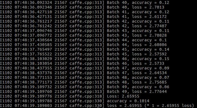
这个测试的准确率明显就很低了,用其他的激活函数试试
具体步骤就不写了,同上
BNLL:

测试:
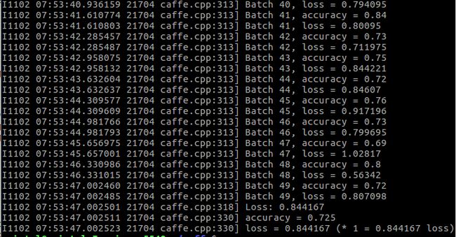
可以看出来这个激活函数和ReLU的效果差不多,比Sigmoid好多了
lr
学习率
caffe中learning rate的polices
    - fixed: always return base_lr.
    - step: return base_lr * gamma ^ (floor(iter / step))
    - exp: return base_lr * gamma ^ iter
    - inv: return base_lr * (1 + gamma * iter) ^ (- power)
    - multistep: similar to step but it allows non uniform steps defined by
      stepvalue
    - poly: the effective learning rate follows a polynomial decay, to be
      zero by the max_iter. return base_lr (1 - iter/max_iter) ^ (power)
    - sigmoid: the effective learning rate follows a sigmod decay
return base_lr ( 1/(1 + exp(-gamma * (iter - stepsize)))) 
修改cifar10中的lr-policy
调整lr大小
根据训练时候运行的文件,我们先看看train_quick.sh文件
#!/usr/bin/env sh
set -e

TOOLS=./build/tools

$TOOLS/caffe train \
  --solver=examples/cifar10/cifar10_quick_solver.prototxt $@


#下面的这个命令可以让cifar10在训练的时候能从上次训练的基础上继续训练
# reduce learning rate by factor of 10 after 8 epochs
$TOOLS/caffe train \
  --solver=examples/cifar10/cifar10_quick_solver_lr1.prototxt \
  --snapshot=examples/cifar10/cifar10_quick_iter_4000.solverstate $@
我们要看调整lr 对训练结果的影响,首先把训练的迭代次数减小到1000
需要将cifar10_quick_solver.prototxt 和cifar10_quick_solver_lr1.prototxt文件修改
# reduce the learning rate after 8 epochs (4000 iters) by a factor of 10

# The train/test net protocol buffer definition
net: "examples/cifar10/cifar10_quick_train_test.prototxt"
# test_iter specifies how many forward passes the test should carry out.
# In the case of MNIST, we have test batch size 100 and 100 test iterations,
# covering the full 10,000 testing images.
test_iter: 100
# Carry out testing every 500 training iterations.
test_interval: 100
# The base learning rate, momentum and the weight decay of the network.
base_lr: 0.001
momentum: 0.9
weight_decay: 0.004
# The learning rate policy
lr_policy: "fixed"
# Display every 100 iterations
display: 100
# The maximum number of iterations
max_iter: 1000
# snapshot intermediate results
snapshot: 1000
snapshot_prefix: "examples/cifar10/models/cifar10_quick"
# solver mode: CPU or GPU
solver_mode: CPU
# reduce the learning rate after 8 epochs (4000 iters) by a factor of 10
# The train/test net protocol buffer definition
net: "examples/cifar10/cifar10_quick_train_test.prototxt"
# test_iter specifies how many forward passes the test should carry out.
# In the case of MNIST, we have test batch size 100 and 100 test iterations,
# covering the full 10,000 testing images.
test_iter: 100
# Carry out testing every 500 training iterations.
test_interval: 100
# The base learning rate, momentum and the weight decay of the network.
base_lr: 0.0001
momentum: 0.9
weight_decay: 0.004
# The learning rate policy
lr_policy: "fixed"
# Display every 100 iterations
display: 100
# The maximum number of iterations
max_iter: 1000
# snapshot intermediate results
snapshot: 1000
snapshot_format: HDF5
snapshot_prefix: "examples/cifar10/cifar10_quick"
# solver mode: CPU or GPU
solver_mode: CPU修改train_quick.sh
#!/usr/bin/env sh
set -e

TOOLS=./build/tools

$TOOLS/caffe train \
  --solver=examples/cifar10/cifar10_quick_solver.prototxt $@

# reduce learning rate by factor of 10 after 8 epochs
$TOOLS/caffe train \
  --solver=examples/cifar10/cifar10_quick_solver_lr1.prototxt \
  --snapshot=examples/cifar10/cifar10_quick_iter_1000.solverstate $@
这样就不用每次都手动降学习率了。
对于大的模型来说,多次降学习率还是很重要的
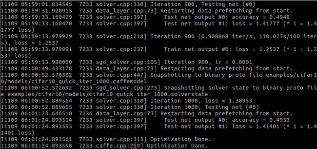
base_lr: 0.001

base_lr:0.0001
base_lr:0.01
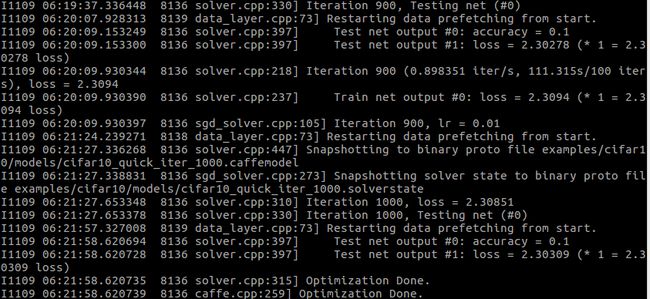
可以明显看出来过大过小都会降低正确率,所以用一个合适的lr也是训练中很重要的一部分.
下面在base_lr:0.001的基础上来修改下lr_policy
# reduce the learning rate after 8 epochs (4000 iters) by a factor of 10

# The train/test net protocol buffer definition
net: "examples/cifar10/cifar10_quick_train_test.prototxt"
# test_iter specifies how many forward passes the test should carry out.
# In the case of MNIST, we have test batch size 100 and 100 test iterations,
# covering the full 10,000 testing images.
test_iter: 100
# Carry out testing every 500 training iterations.
test_interval: 100
# The base learning rate, momentum and the weight decay of the network.
base_lr: 0.001
momentum: 0.9
weight_decay: 0.004
# The learning rate policy
lr_policy: "step"
stepsize:100
gamma:0.1
# Display every 100 iterations
display: 100
# The maximum number of iterations
max_iter: 1000
# snapshot intermediate results
snapshot: 1000
snapshot_prefix: "examples/cifar10/models/cifar10_quick"
# solver mode: CPU or GPU
solver_mode: CPU
dropout
dropout类型
正向dropout、反向dropout。
反向Dropout有助于只定义一次模型并且只改变了一个参数(保持/丢弃概率)以使用同一模型进行训练和测试。相反,直接Dropout,迫使你在测试阶段修改网络。因为如果你不乘以比例因子q,神经网络的输出将产生更高的相对于连续神经元所期望的值(因此神经元可能饱和):这就是为什么反向Dropout是更加常见的实现方式。
正向Dropout:通常与L2正则化和其它参数约束技术(如Max Norm1)一起使用。正则化有助于保持模型参数值在可控范围内增长。
反向Dropout:学习速率被缩放至q的因子,我们将其称q为推动因子(boosting factor),因为它推动了学习速率。此外,我们将r(q)称为有效学习速率(effective learning rate)。总之,有效学习速率相对于所选择的学习速率更高:由于这个原因,限制参数值的正则化可以帮助简化学习速率选择过程
缺点
- Dropout是一个正则化技术,它减少了模型的有效容量
- 只有极少的训练样本可用时,Dropout不会很有效
在cifar实例中加入dropout
layer {
  name:"drop1"
  type:"Dropout"
  bottom:""#这里填下一层
  top:""#这里填上一层
  dropout_param {
    dropout_ratio:0.5
  }
}
batch normalization
对于每一组batch,在网络的每一层中,分feature对输入进行normalization,对各个feature分别normalization,即对网络中每一层的单个神经元输入,计算均值和方差后,再进行normalization。
cifar10中的BatchNorm
use_global_stats==true时会强制使用模型中存储的BatchNorm层均值与方差参数,而非基于当前batch内计算均值和方差。
batch normalization的主要目的是改善优化,但噪音具有正则化的效果,有时使Dropout变得没有必要。
data augmentation
有的时候训练集不够用,或者某一类数据较少,或者为了防止过拟合,可以用data augmentation对已有的数据集进行操作
常见方法
Color Jittering:对颜色的数据增强:图像亮度、饱和度、对比度变化(此处对色彩抖动的理解不知是否得当);

PCA Jittering:首先按照RGB三个颜色通道计算均值和标准差,再在整个训练集上计算协方差矩阵,进行特征分解,得到特征向量和特征值,用来做PCA Jittering;

Random Scale:尺度变换;

Random Crop:采用随机图像差值方式,对图像进行裁剪、缩放;包括Scale Jittering方法(VGG及ResNet模型使用)或者尺度和长宽比增强变换;

Horizontal/Vertical Flip:水平/垂直翻转;

Shift:平移变换;

Rotation/Reflection:旋转/仿射变换;

Noise:高斯噪声、模糊处理;

Label shuffle:类别不平衡数据的增广,参见海康威视ILSVRC2016的report;另外,文中提出了一种Supervised Data Augmentation方法,有兴趣的朋友的可以动手实验下。
cifar10中的
 transform_param {
    mean_file: #均值文件
    scale:#像素归一化
    mirror: true#训练集会randomly mirrors the input image
    crop_size: #train时会对大于crop_size的图片进行随机裁剪,而在test时只是截取中间部分
  }
参考文章:
http://www.cnblogs.com/maohai/p/6453417.html
http://blog.csdn.net/u010402786/article/details/51233854