推荐系统初学者系列（6）-- TSNE

上一篇：推荐系统初学者系列（5）– 混合推荐机制
下一篇：推荐系统初学者系列（7）–Surprise库做Top-K推荐

介绍

许多数据科学家经常面对的问题之一：假设有一个包含数百个特征（变量）的数据集，且对数据所属的域没有任何了解，需要对该数据集识别其隐藏状态、探索并分析。本文将介绍一种非常强大的方法来解决该问题。

1 什么是t-SNE

（t-SNE）t分布随机邻域嵌入 是一种用于探索高维数据的非线性降维算法。它将多维数据映射到适合于人类观察的两个或多个维度。

2 什么是降维？

简而言之，降维就是用2维或3维表示多维数据（彼此具有相关性的多个特征数据）的技术，利用降维算法，可以显式地表现数据。

PCA的局限性

PCA是一种线性算法，它不能解释特征之间的复杂多项式关系。而t-SNE是基于在邻域图上随机游走的概率分布来找到数据内的结构。

线性降维算法的一个主要问题是不相似的数据点放置在较低维度表示为相距甚远。但为了在低维度用非线性流形表示高维数据，相似数据点必须表示为非常靠近，这不是线性降维算法所能做的。

3 t-SNE实际上是做什么？

t-SNE非线性降维算法通过基于具有多个特征的数据点的相似性识别观察到的簇来在数据中找到模式。本质上是一种降维和可视化技术。另外t-SNE的输出可以作为其他分类算法的输入特征。

4 python代码演示

# -*- coding:utf-8 -*-

from time import time
import numpy as np
import matplotlib.pyplot as plt
from matplotlib import offsetbox
from sklearn import (manifold, datasets, decomposition, ensemble,
                     discriminant_analysis, random_projection)

## Loading and curating the data
digits = datasets.load_digits(n_class=10)
X = digits.data
y = digits.target
n_samples, n_features = X.shape
n_neighbors = 30


## Function to Scale and visualize the embedding vectors
def plot_embedding(X, title=None):
    x_min, x_max = np.min(X, 0), np.max(X, 0)
    X = (X - x_min) / (x_max - x_min)
    plt.figure()
    ax = plt.subplot(111)
    for i in range(X.shape[0]):
        plt.text(X[i, 0], X[i, 1], str(digits.target[i]),
                 color=plt.cm.Set1(y[i] / 10.),
                 fontdict={'weight': 'bold', 'size': 9})
    if hasattr(offsetbox, 'AnnotationBbox'):
        ## only print thumbnails with matplotlib > 1.0
        shown_images = np.array([[1., 1.]])  # just something big
        for i in range(digits.data.shape[0]):
            dist = np.sum((X[i] - shown_images) ** 2, 1)
            if np.min(dist) < 4e-3:
                ## don't show points that are too close
                continue
            shown_images = np.r_[shown_images, [X[i]]]
            imagebox = offsetbox.AnnotationBbox(
                offsetbox.OffsetImage(digits.images[i], cmap=plt.cm.gray_r),
                X[i])
            ax.add_artist(imagebox)
    plt.xticks([]), plt.yticks([])
    if title is not None:
        plt.title(title)


# ----------------------------------------------------------------------
## Plot images of the digits
n_img_per_row = 20
img = np.zeros((10 * n_img_per_row, 10 * n_img_per_row))
for i in range(n_img_per_row):
    ix = 10 * i + 1
    for j in range(n_img_per_row):
        iy = 10 * j + 1
        img[ix:ix + 8, iy:iy + 8] = X[i * n_img_per_row + j].reshape((8, 8))
plt.imshow(img, cmap=plt.cm.binary)
plt.xticks([])
plt.yticks([])
plt.title('A selection from the 64-dimensional digits dataset')
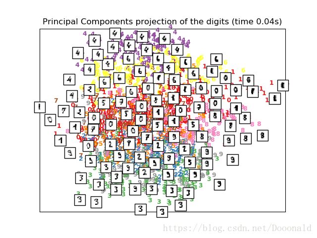
## Computing PCA
print("Computing PCA projection")
t0 = time()
X_pca = decomposition.TruncatedSVD(n_components=2).fit_transform(X)
plot_embedding(X_pca,
               "Principal Components projection of the digits (time %.2fs)" %
               (time() - t0))
## Computing t-SNE
print("Computing t-SNE embedding")
tsne = manifold.TSNE(n_components=2, init='pca', random_state=0)
t0 = time()
X_tsne = tsne.fit_transform(X)
plot_embedding(X_tsne,
               "t-SNE embedding of the digits (time %.2fs)" %
               (time() - t0))
plt.show()