斯坦福大学机器学习公开课---Programming Exercise 2: Logistic Regression
斯坦福大学机器学习公开课---Programming Exercise 2: Logistic Regression---Matlab实现
1 Logistic Regression
In this part of the exercise, I will build a logistic regression model to predict whether a student gets admitted into a university.
You want to determine each applicant’s chance of admission based on their scores on two exams.
1.1 Visualizing the data
function plotData(X, y)
%PLOTDATA Plots the data points X and y into a new figure
%   PLOTDATA(x,y) plots the data points with + for the positive examples
%   and o for the negative examples. X is assumed to be a Mx2 matrix.

% Create New Figure
figure; hold on;

% ====================== YOUR CODE HERE ======================
% Instructions: Plot the positive and negative examples on a
%               2D plot, using the option 'k+' for the positive
%               examples and 'ko' for the negative examples.


% Find Indices of Positive and Negative Examples
pos = find(y==1); neg = find(y == 0);  % 对应0/1的相应地址向量
% Plot Examples
plot(X(pos, 1), X(pos, 2), 'k+','LineWidth', 2, ...
'MarkerSize', 7);
plot(X(neg, 1), X(neg, 2), 'ko', 'MarkerFaceColor', 'y', ...
'MarkerSize', 7);

% =========================================================================


hold off;

end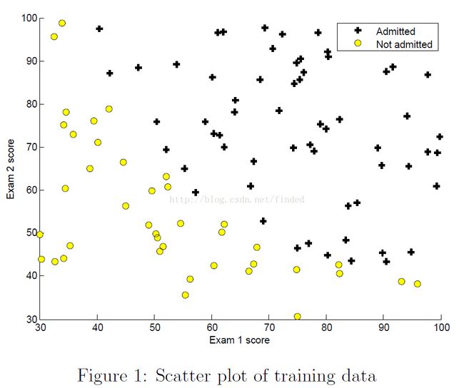
1.2 Plotting the decision boundary
plotDecisionBoundary.m using the θ value to plot a Decision boundary.注意:决策边界只与假设h的形式和theta的值有关,给定假设h和theta就可以得到决策边界;而与训练序列无关。
function plotDecisionBoundary(theta, X, y)
%PLOTDECISIONBOUNDARY Plots the data points X and y into a new figure with
%the decision boundary defined by theta
%   PLOTDECISIONBOUNDARY(theta, X,y) plots the data points with + for the
%   positive examples and o for the negative examples. X is assumed to be
%   a either
%   1) Mx3 matrix, where the first column is an all-ones column for the
%      intercept.
%   2) MxN, N>3 matrix, where the first column is all-ones

% Plot Data
plotData(X(:,2:3), y);
hold on


if size(X, 2) <= 3  %feature =1,2,
    % Only need 2 points to define a line, so choose two endpoints 端点
    plot_x = [min(X(:,2))-2,  max(X(:,2))+2];% 两点横坐标,第一个特征的最大最小值,横坐标的始末地址-+2。

    % Calculate the decision boundary line
    plot_y = (-1./theta(3)).*( theta(2).*plot_x + theta(1)); %第二个特征的预测值???p=0.5,决策边界 theta*X=0

    % Plot, and adjust axes for better viewing
    plot(plot_x, plot_y)

    % Legend, specific for the exercise
    legend('Admitted', 'Not admitted', 'Decision Boundary')
    axis([30, 100, 30, 100])


else  %
    % Here is the grid range
    u = linspace(-1, 1.5, 50); % -1->1.5 区间50 等分取点
    v = linspace(-1, 1.5, 50);

    z = zeros(length(u), length(v));
    % Evaluate z = theta*x over the grid
    for i = 1:length(u)
        for j = 1:length(v)
            z(i,j) = mapFeature(u(i), v(j))*theta;
        end
    end
    z = z'; % important to transpose z before calling contour

    % Plot z = 0
    % Notice you need to specify the range [0, 0]
    contour(u, v, z, [0, 0], 'LineWidth', 2)%???
end
hold off

end


% MAPFEATURE Feature mapping function to polynomial features
  % MAPFEATURE(X1, X2) maps the two input features
  % to quadratic features used in the regularization exercise.

  % Returns a new feature array with more features, comprising of
  % X1, X2, X1.^2, X2.^2, X1*X2, X1*X2.^2, etc..

  % Inputs X1, X2 must be the same size
1.2 Implementation
1.2.1 Warmup exercise: sigmoid function
The logistic regression hypothesis is :
For a matrix, the SIGMOID function perform the sigmoid function on every element.
function g = sigmoid(z)
%SIGMOID Compute sigmoid functoon
%   J = SIGMOID(z) computes the sigmoid of z.

% You need to return the following variables correctly
g = zeros(size(z));

% ====================== YOUR CODE HERE ======================
% Instructions: Compute the sigmoid of each value of z (z can be a matrix,
%               vector or scalar).

g = 1./(ones(size(z))+e.^(-z));

% =============================================================

end
1.2.2 Cost function and gradient
Cost
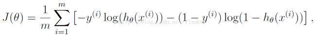
Gradient

The costFunction function implement the cost function and gradient for logistic regression, return the cost and gradient.
function [J, grad] = costFunctionReg(theta, X, y, lambda)
%COSTFUNCTIONREG Compute cost and gradient for logistic regression with regularization
%   J = COSTFUNCTIONREG(theta, X, y, lambda) computes the cost of using
%   theta as the parameter for regularized logistic regression and the
%   gradient of the cost w.r.t. to the parameters.

% Initialize some useful values
m = length(y); % number of training examples

n = length(theta);
% You need to return the following variables correctly
J = 0;
grad = zeros(size(theta));

% ====================== YOUR CODE HERE ======================
% Instructions: Compute the cost of a particular choice of theta.
%               You should set J to the cost.
%               Compute the partial derivatives and set grad to the partial
%               derivatives of the cost w.r.t. each parameter in theta


predictions = sigmoid(X*theta);         % m x 1 predictions of hypothesis on all m examples
J = 1/m *(-y'*log(predictions)-(1-y)'*log(1-predictions)) + 1/(2*m)*lambda*(theta'*theta-(theta(1,1))^2);   % cost function


grad(1,1) = (1/m *(predictions-y)'*X(:,1));
%size(grad(2:n,1));
%(1/m *lambda*theta(2:n,1))
grad(2:n,1) = (1/m *(predictions-y)'*X(:,2:n) )'+ 1/m *lambda*theta(2:n,1);%+


% =============================================================

end
1.2.3 Learning parameters using fminunc
Octave’s fminunc is an optimization solver that finds the minimum of an unconstrained function.
You will pass to fminunc the following inputs:
- The initial values of the parameters we are trying to optimize
- A function that, when given the training set and a particular theta, computes the logistic regressioncost and gradient with respect to theta for the dataset(X, y)
%% Machine Learning Online Class - Exercise 2: Logistic Regression
%
%  Instructions
%  ------------
%
%  This file contains code that helps you get started on the logistic
%  regression exercise. You will need to complete the following functions
%  in this exericse:
%
%     sigmoid.m
%     costFunction.m
%     predict.m
%     costFunctionReg.m
%
%  For this exercise, you will not need to change any code in this file,
%  or any other files other than those mentioned above.
%


%% Initialization
clear ; close all; clc


%% Load Data
%  The first two columns contains the exam scores and the third column
%  contains the label.


data = load('ex2data1.txt');
X = data(:, [1, 2]); y = data(:, 3);


%% ==================== Part 1: Plotting ====================
%  We start the exercise by first plotting the data to understand the
%  the problem we are working with.


fprintf(['Plotting data with + indicating (y = 1) examples and o ' ...
         'indicating (y = 0) examples.\n']);


plotData(X, y);


% Put some labels
hold on;
% Labels and Legend
xlabel('Exam 1 score')
ylabel('Exam 2 score')


% Specified in plot order
legend('Admitted', 'Not admitted')
hold off;


fprintf('\nProgram paused. Press enter to continue.\n');
pause;


%% ============ Part 2: Compute Cost and Gradient ============
%  In this part of the exercise, you will implement the cost and gradient
%  for logistic regression. You neeed to complete the code in
%  costFunction.m


%  Setup the data matrix appropriately, and add ones for the intercept term
[m, n] = size(X);


% Add intercept term to x and X_test
X = [ones(m, 1) X];


% Initialize fitting parameters
initial_theta = zeros(n + 1, 1);


% Compute and display initial cost and gradient
[cost, grad] = costFunction(initial_theta, X, y);
fprintf('Cost at initial theta (zeros): %f\n', cost);
fprintf('Gradient at initial theta (zeros): \n');
fprintf(' %f \n', grad);


fprintf('\nProgram paused. Press enter to continue.\n');
pause;


%% ============= Part 3: Optimizing using fminunc  =============
%  In this exercise, you will use a built-in function (fminunc) to find the
%  optimal parameters theta.


%  Set options for fminunc
options = optimset('GradObj', 'on', 'MaxIter', 400);


%  Run fminunc to obtain the optimal theta
%  This function will return theta and the cost
[theta, cost] = ...
	fminunc(@(t)(costFunction(t, X, y)), initial_theta, options);


% Print theta to screen
fprintf('Cost at theta found by fminunc: %f\n', cost);
fprintf('theta: \n');
fprintf(' %f \n', theta);


% Plot Boundary
plotDecisionBoundary(theta, X, y);


% Put some labels
hold on;
% Labels and Legend
xlabel('Exam 1 score')
ylabel('Exam 2 score')


% Specified in plot order
legend('Admitted', 'Not admitted')
hold off;


fprintf('\nProgram paused. Press enter to continue.\n');
pause;


%% ============== Part 4: Predict and Accuracies ==============
%  After learning the parameters, you'll like to use it to predict the outcomes
%  on unseen data. In this part, you will use the logistic regression model
%  to predict the probability that a student with score 45 on exam 1 and
%  score 85 on exam 2 will be admitted.
%
%  Furthermore, you will compute the training and test set accuracies of
%  our model.
%
%  Your task is to complete the code in predict.m


%  Predict probability for a student with score 45 on exam 1
%  and score 85 on exam 2


prob = sigmoid([1 45 85] * theta);
fprintf(['For a student with scores 45 and 85, we predict an admission ' ...
         'probability of %f\n\n'], prob);


% Compute accuracy on our training set
p = predict(theta, X);


fprintf('Train Accuracy: %f\n', mean(double(p == y)) * 100);


fprintf('\nProgram paused. Press enter to continue.\n');
pause;

2 Regularizedlogistic regression
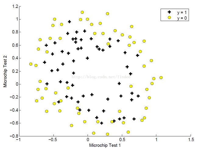
It will implement regularized logistic regression to predict whether microchips from afabrication plant passes quality assurance(QA).
2.1 Visualizing the data
2.2 Featuremapping
One way to fit the data better is to create more features from each data point. In the provided function mapFeature.m, we will map the 2 features into 28 polynomial terms of x1 and x2 up to the sixth power.

function out = mapFeature(X1, X2)
% MAPFEATURE Feature mapping function to polynomial features
%
% MAPFEATURE(X1, X2) maps the two input features
% to quadratic features used in the regularization exercise.
%
% Returns a new feature array with more features, comprising of
% X1, X2, X1.^2, X2.^2, X1*X2, X1*X2.^2, etc..
%
% Inputs X1, X2 must be the same size
%
degree = 6;
out = ones(size(X1(:,1)));
for i = 1:degree
for j = 0:i
out(:, end+1) = (X1.^(i-j)).*(X2.^j);
end
end
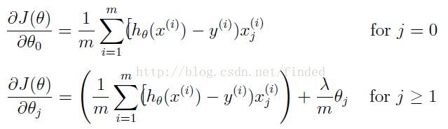
end2.3 Cost function and gradient
Now i will implement code to compute the cost function and gradient for regularized logistic regression to avoid overfitting.cost function
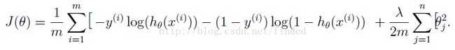
gradient
function [J, grad] = costFunctionReg(theta, X, y, lambda)
%COSTFUNCTIONREG Compute cost and gradient for logistic regression with regularization
%   J = COSTFUNCTIONREG(theta, X, y, lambda) computes the cost of using
%   theta as the parameter for regularized logistic regression and the
%   gradient of the cost w.r.t. to the parameters.

% Initialize some useful values
m = length(y); % number of training examples

n = length(theta);
% You need to return the following variables correctly
J = 0;
grad = zeros(size(theta));

% ====================== YOUR CODE HERE ======================
% Instructions: Compute the cost of a particular choice of theta.
%               You should set J to the cost.
%               Compute the partial derivatives and set grad to the partial
%               derivatives of the cost w.r.t. each parameter in theta


predictions = sigmoid(X*theta);         % m x 1 predictions of hypothesis on all m examples
J = 1/m *(-y'*log(predictions)-(1-y)'*log(1-predictions)) + 1/(2*m)*lambda*(theta'*theta-(theta(1,1))^2);   % cost function


grad(1,1) = (1/m *(predictions-y)'*X(:,1));
%size(grad(2:n,1));
%(1/m *lambda*theta(2:n,1))
grad(2:n,1) = (1/m *(predictions-y)'*X(:,2:n) )'+ 1/m *lambda*theta(2:n,1);%+


% =============================================================

end
2.5 Optional (ungraded) exercises
%% Machine Learning Online Class - Exercise 2: Logistic Regression
%
% Instructions
% ------------
%
% This file contains code that helps you get started on the second part
% of the exercise which covers regularization with logistic regression.
%
% You will need to complete the following functions in this exericse:
%
% sigmoid.m
% costFunction.m
% predict.m
% costFunctionReg.m
%
% For this exercise, you will not need to change any code in this file,
% or any other files other than those mentioned above.
%
%% Initialization
clear ; close all; clc
%% Load Data
% The first two columns contains the X values and the third column
% contains the label (y).
data = load('ex2data2.txt');
X = data(:, [1, 2]); y = data(:, 3);
plotData(X, y);
% Put some labels
hold on;
% Labels and Legend
xlabel('Microchip Test 1')
ylabel('Microchip Test 2')
% Specified in plot order
legend('y = 1', 'y = 0')
hold off;
%% =========== Part 1: Regularized Logistic Regression ============
% In this part, you are given a dataset with data points that are not
% linearly separable. However, you would still like to use logistic
% regression to classify the data points.
%
% To do so, you introduce more features to use -- in particular, you add
% polynomial features to our data matrix (similar to polynomial
% regression).
%
% Add Polynomial Features
% Note that mapFeature also adds a column of ones for us, so the intercept
% term is handled
%size(X)
X = mapFeature(X(:,1), X(:,2));
%size(X)
% Initialize fitting parameters
initial_theta = zeros(size(X, 2), 1);
% Set regularization parameter lambda to 1
lambda = 1;
% Compute and display initial cost and gradient for regularized logistic
% regression
[cost, grad] = costFunctionReg(initial_theta, X, y, lambda);
fprintf('Cost at initial theta (zeros): %f\n', cost);
fprintf('\nProgram paused. Press enter to continue.\n');
pause;
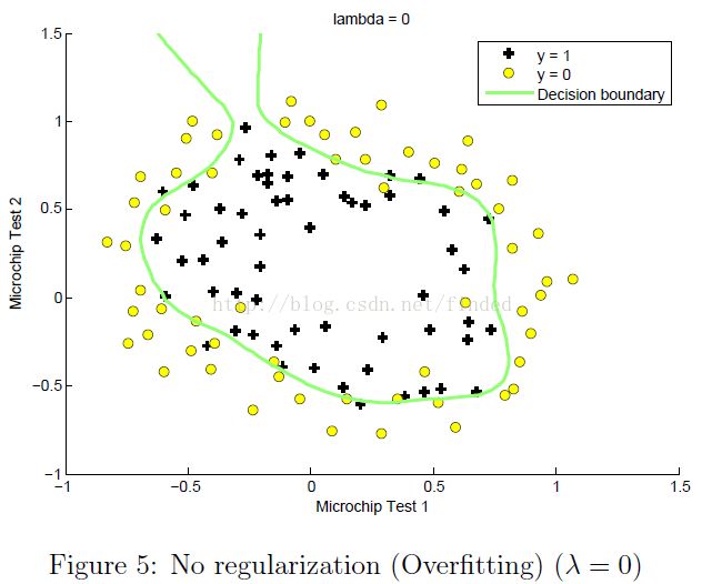
%% ============= Part 2: Regularization and Accuracies =============
% Optional Exercise:
% In this part, you will get to try different values of lambda and
% see how regularization affects the decision coundart
%
% Try the following values of lambda (0, 1, 10, 100).
%
% How does the decision boundary change when you vary lambda? How does
% the training set accuracy vary?
%
% Initialize fitting parameters
initial_theta = zeros(size(X, 2), 1);
% Set regularization parameter lambda to 1 (you should vary this)
lambda = 1;
% Set Options
options = optimset('GradObj', 'on', 'MaxIter', 400);
% Optimize
[theta, J, exit_flag] = ...
fminunc(@(t)(costFunctionReg(t, X, y, lambda)), initial_theta, options);
% Plot Boundary
plotDecisionBoundary(theta, X, y);
hold on;
title(sprintf('lambda = %g', lambda))
% Labels and Legend
xlabel('Microchip Test 1')
ylabel('Microchip Test 2')
legend('y = 1', 'y = 0', 'Decision boundary')
hold off;
% Compute accuracy on our training set
p = predict(theta, X);
fprintf('Train Accuracy: %f\n', mean(double(p == y)) * 100);