机器学习基石 5.3 Effective Number of Hypotheses
文章目录
- 1. Dichotomies: Mini-hypotheses
- 2. Growth Function
- 3. Growth Function for Positive Rays
- 4. Growth Function for Positive Intervals
- 5. Growth Function for Convex Sets
- 6. Fun Time
1. Dichotomies: Mini-hypotheses
原来的hypothesis set:

引入新概念:
dichotomy:只关注hypothesis作用在 x 1 , x 2 , ⋯ , x N \mathbf{x_{1}},\mathbf{x_{2}},\cdots,\mathbf{x_{N}} x1,x2,⋯,xN上的结果,这样就可以把所有的hypothesis像上一节一样进行分类。
![]()
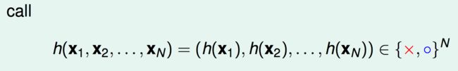
令
h ( x 1 , x 2 , ⋯ , x N ) = ( h ( x 1 ) , h ( x 2 ) , ⋯ , h ( x N ) ) ∈ { × , ◯ } N h(\mathbf{x_{1}},\mathbf{x_{2}},\cdots,\mathbf{x_{N}})=(h(\mathbf{x_{1}}),h(\mathbf{x_{2}}),\cdots,h(\mathbf{x_{N}})) \in \{\times ,\bigcirc\}^N h(x1,x2,⋯,xN)=(h(x1),h(x2),⋯,h(xN))∈{×,◯}N
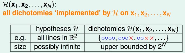
希望可以用 ∣ H ( x 1 , x 2 , ⋯ , x N ) ∣ |\mathcal{H}(\mathbf{x_{1}},\mathbf{x_{2}},\cdots,\mathbf{x_{N}})| ∣H(x1,x2,⋯,xN)∣来代替原来的 M M M。
![]()
2. Growth Function
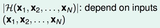
然而 ∣ H ( x 1 , x 2 , ⋯ , x N ) ∣ |\mathcal{H}(\mathbf{x_{1}},\mathbf{x_{2}},\cdots,\mathbf{x_{N}})| ∣H(x1,x2,⋯,xN)∣与输入的 ( x 1 , x 2 , ⋯ , x N ) (\mathbf{x_{1}},\mathbf{x_{2}},\cdots,\mathbf{x_{N}}) (x1,x2,⋯,xN)有关。
用其最大值来摆脱输入的依赖。

比如:
m H ( 1 ) = 2 m_{H}(1) =2 mH(1)=2
m H ( 2 ) = 4 m_{H}(2) =4 mH(2)=4
m H ( 3 ) = 8 m_{H}(3) =8 mH(3)=8
m H ( 4 ) = 14 m_{H}(4) =14 mH(4)=14

3. Growth Function for Positive Rays
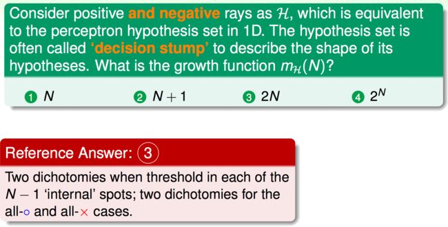
考虑一个简单的情况:Positive Rays
h ( x ) = { 1 , x > t h r e s h o l d − 1 , x ⩽ t h r e s h o l d h(x) = \begin{cases} 1, &x>threshold\\ -1, &x\leqslant threshold \end{cases} h(x)={1,−1,x>thresholdx⩽threshold

相当于一维的perceptrons的一半。

易得

H ( x 1 , x 2 , ⋯ , x N ) \mathcal{H}(\mathbf{x_{1}},\mathbf{x_{2}},\cdots,\mathbf{x_{N}}) H(x1,x2,⋯,xN)中每一个 h ( x 1 , x 2 , ⋯ , x N ) \mathcal{h}(\mathbf{x_{1}},\mathbf{x_{2}},\cdots,\mathbf{x_{N}}) h(x1,x2,⋯,xN)的样子

当 N N N很大时, N + 1 N+1 N+1远小于 2 N 2^N 2N。

4. Growth Function for Positive Intervals
考虑另外一种情况:Positive Intervals
范围内为+1,范围外为-1。

它的 m H ( N ) m_{H}(N) mH(N)
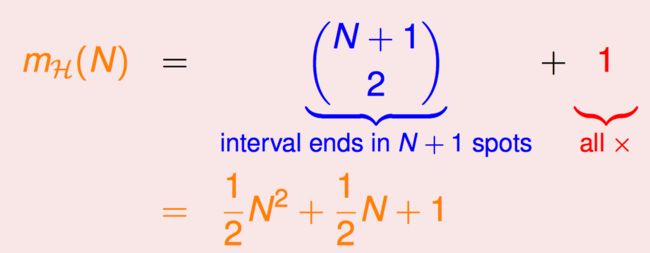
N N N个点把数轴分为 N + 1 N+1 N+1段,如果范围的两个端点放在不同的段内,那么一共有$
\begin{pmatrix}
N+1 \
2 \
\end{pmatrix}
$种,如果放在同一段内,那么只有1种。
H ( x 1 , x 2 , ⋯ , x N ) \mathcal{H}(\mathbf{x_{1}},\mathbf{x_{2}},\cdots,\mathbf{x_{N}}) H(x1,x2,⋯,xN)中每一个 h ( x 1 , x 2 , ⋯ , x N ) \mathcal{h}(\mathbf{x_{1}},\mathbf{x_{2}},\cdots,\mathbf{x_{N}}) h(x1,x2,⋯,xN)的样子

这个结果在 N N N很大时也是远小于 2 N 2^N 2N的。

5. Growth Function for Convex Sets
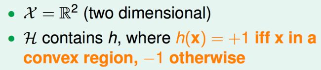
考虑 h h h为平面上的一个凸包的情况
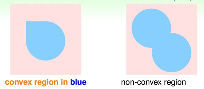
当 x \mathbf{x} x在凸包内部时, h ( x ) = 1 h(\mathbf{x})=1 h(x)=1,否则 h ( x ) = − 1 h(\mathbf{x})=-1 h(x)=−1
一种可能的输入:所有的点都在一个大圆上。
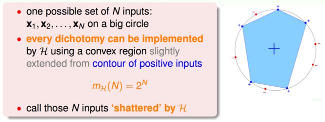
这时无论每个点对应的是圈还是叉,都能找到一种凸包对应一个dichotomy。

6. Fun Time