CS231n课程作业(一) SVM classifier

一、理论知识

1. score function

将原始数据映射到每一类上计算得分的函数。
(PS: CNN也是将原始输入的像素映射成类目得分，只不过其中间映射更加复杂，参数更多。)
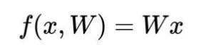
对于SVM，score function为：

其中，xi指第i张图片，W为权重(可以理解为图像上每个像素点都有weight)，b为偏移量bias。
这里可以看出，优化时不仅要调整W，还需调整b。为了简化优化，将b并入到W中，形成一个新的W，这样优化时只需对W优化即可。处理方法如下：

因此，新的score function为：

2. loss function

用于描述模型预测值与真实值的不一致程度。
loss function is made of two component: data loss and regularization loss.
data loss为：

其中，Li表示第i张图片的data loss， sj指第i张图片对第j类的score，syi指第i张图片所属正确类的score。这里的1其实是一个给定的delta值，也可以设为其他常数，delta的含义是正确类的score不仅理应比其他类的score高，而且应该高出delta，否则将产生data loss。
训练模型的目的就是让loss值最小，即optimization。
Optimization： start with a random W and find a W that minimizes the loss.
但是，有时多组W可以得到相同的data loss值，比如：

这样W就是不确定的。因此，需要通过正则化选取一组最合适的W。
Regularization loss :(in common use: L2 regularization)

因此，完整的loss function为：

其中，N为训练样本的数量，lambda为正则项系数。lambda由cross-validation确定。(还有learning rate)

3. 梯度相关知识

梯度：指loss function对W求导，这样可以得到函数下降最快的方向。
numerical gradient: 即从求导的定义出发

analytic gradient: 直接用Li对W求偏导
numerical gradient is easy to write but slow and approximate, and analytic gradient is fast and exact but error-prone. In practice, derive analytic gradient, then check your implementation with numerical gradient.
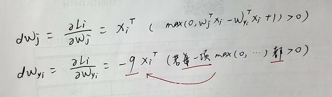
这是data loss 的展开形式：

其中，Li指第i张图片的data loss值，Wj指W矩阵的第j列(即权重矩阵对第j类的权)，Wyi指W矩阵的第yi列(权重矩阵对第i张图片的正确所属类的权)。本作业中：W:(3073,10), X:(N,3073), y:(N,)
这里变量是W，求analytic gradient：
(更新：下面为错解，正解见下面的更新)

———————————————————————2018-1-10更新——————————————————————

————————————————————————–更新完毕———————————————————————–

*注：这两种梯度求法在编写svm classifier中很关键！

梯度下降： 梯度下降即通过反复的迭代运算，计算gradient进行权值更新，最后停留在loss function的低值点。(此时的W是使loss function最低的W。)

作一个直观理解：比如你半夜小便，眼睛睁不开，不开灯，对着马桶开始飙尿。你的目的是尽快(因为尿量总共就那么多)尿到马桶中有水的区域。所以你开始randomly尿到一侧马桶内壁，然后不断的下降落尿点。这里你需要get到最快的下降方向，也就是gradient，沿着这个梯度负方向下降一定的步长(step_size或learning rate)，一点一点的尿到马桶的最低点。此时对卫生间的环境损失最小(minimize the loss function)，然后你按下冲水按钮，就可以安心睡觉了。

4. 迭代相关知识

batch_size: number of training examples to use at each iteration.
迭代的具体工作：
(1) 取batch_size个样本，evaluate the loss & gradient.
(2) update W: W += -learning_rate * gradient
(3) 利用更新好的W，重复(1)、(2)，直到迭代结束。

Mini-batch Gradient Descent: In practice, only use a small portion of the training set to compute the gradient of loss function.
缺点：得出的gradient很有可能是一个噪声
优点：使用小样本计算可以提高运算速度，可以计算更多的次数来evaluate gradient，从而得出最低的loss function。或者也可以降低运算循环次数，使用更加精确的gradient。另外，在实际中使用所有数据计算梯度并不可行。(GPU hold不住)

learning_rate: 每一次迭代中W沿梯度负方向移动的大小(见上面“迭代的具体工作”)，lr决定了参数移动到最优值的速度快慢。lr的值由cross-validation确定。(还有正则项系数lambda也是)
if very high: loss function不会收敛，会越来越大。
if high: loss function会收敛，但可能收敛后的函数值会越过最优值，卡在一个比较高的位置，即没有找到最低的loss function。由于更新速度快，你不能确定要优化的函数是否进入一个局部最小值，你以为局部最小值是最小值，但实际并不是。
if low: 更新速度慢，收敛需要很长时间。
if good: then good.
策略：先set a high lr，再一点点降低。

二、SVM classifier

1. 数据介绍

50000张图片，32x32x3， 10类。其中training set为49000张， test set为1000张。
从training set中产生validation set 1000张和development set 500张。
X_train: (49000,3072) , y_train: (49000,)
X_val: (1000,3072) , y_val: (1000,)
X_test: (1000,3072) , y_test: (1000,)
X_dev: (500,3072) , y_dev: (500,)
*以上3072在运算中均增加为3073，原因不解释(除非你没好好看上面的理论部分)
W: (3073,10)
dW: (3073,10)

2. 预处理: 去均值

这样的处理其实很常见，例如摄影测量里的重心化。
first: compute the image mean based on the training data
second: subtract the mean image from train and test data
third: append the bias dimension of ones (i.e. bias trick) so that our SVM only has to worry about optimizing a single weight matrix W.

3. 计算loss和梯度

这里的梯度是analytic gradient
方法一 naive版：

def svm_loss_naive(W, X, y, reg):
  """
  Structured SVM loss function, naive implementation (with loops).

  Inputs have dimension D, there are C classes, and we operate on minibatches
  of N examples.

  Inputs:
  - W: A numpy array of shape (D, C) containing weights.
  - X: A numpy array of shape (N, D) containing a minibatch of data.
  - y: A numpy array of shape (N,) containing training labels; y[i] = c means
    that X[i] has label c, where 0 <= c < C.
  - reg: (float) regularization strength

  Returns a tuple of:
  - loss as single float
  - gradient with respect to weights W; an array of same shape as W
  """
  dW = np.zeros(W.shape) # initialize the gradient as zero (3073,10)

  # compute the loss and the gradient
  num_classes = W.shape[1]    #10类
  num_train = X.shape[0]      # 500个训练样本
  loss = 0.0
  for i in xrange(num_train):
    scores = X[i].dot(W)        # (1,10)
    correct_class_score = scores[y[i]] #第y[i]类的得分 或 第i个样本的所属类别的得分
    for j in xrange(num_classes):
      if j == y[i]:
        continue            #跳出当前循环，执行下一次循环
      margin = scores[j] - correct_class_score + 1 # note delta = 1
      if margin > 0:
        loss += margin          #计算data loss
        dW[:,j] += X[i].T       # dW: 3073x10, 此处的值为3073x1,放在dW第j列，dW[:,j]只需加一次，外循环再循环500次
        dW[:,y[i]] += -X[i].T   #dW[:,y[i]要加9次]，除非有margin<0;外循环再循环500次
  # Right now the loss is a sum over all training examples, but we want it
  # to be an average instead so we divide by num_train.
  loss /= num_train         #由于样本太多，loss值累积，所以取均值
  dW /= num_train
  # Add regularization to the loss.
  loss += reg * np.sum(W * W)       # L2 regularization
  dW += reg * W
  #############################################################################
  # TODO:                                                                     #
  # Compute the gradient of the loss function and store it dW.                #
  # Rather that first computing the loss and then computing the derivative,   #
  # it may be simpler to compute the derivative at the same time that the     #
  # loss is being computed. As a result you may need to modify some of the    #
  # code above to compute the gradient.                                       #
  #############################################################################


  return loss, dW

方法二 矢量化版：

def svm_loss_vectorized(W, X, y, reg):
  """
  Structured SVM loss function, vectorized implementation.

  Inputs and outputs are the same as svm_loss_naive.
  """
  loss = 0.0
  dW = np.zeros(W.shape) # initialize the gradient as zero

  #############################################################################
  # TODO:                                                                     #
  # Implement a vectorized version of the structured SVM loss, storing the    #
  # result in loss.                                                           #
  #############################################################################
  scores = X.dot(W)
  correct = []
  for i in xrange(X.shape[0]):
    correct.append(scores[i,y[i]])
  #或： correct = scores[range(500),list(y)]
  correct = np.mat(correct).T
  margin = np.maximum(0,scores - correct + 1) 
  loss = np.sum(margin) + np.sum(correct) - X.shape[0]  #将上面naive中j==y[i]多减多加的部分还原
  #处理2：也可以将j==y[i]的项置0
  #即：margin[range(500),list(y)]=0
  loss = loss/X.shape[0]
  loss += reg * np.sum(W * W)
  #############################################################################
  #                             END OF YOUR CODE                              #
  #############################################################################


  #############################################################################
  # TODO:                                                                     #
  # Implement a vectorized version of the gradient for the structured SVM     #
  # loss, storing the result in dW.                                           #
  #                                                                           #
  # Hint: Instead of computing the gradient from scratch, it may be easier    #
  # to reuse some of the intermediate values that you used to compute the     #
  # loss.                                                                     #
  #############################################################################
  coeff = np.zeros(margin.shape) #500x10
  coeff[margin>0]=1  #置1的目的是dWj这一项，让所有样本的Xi相加;而margin<0时不计入loss，所以置0
  coeff[range(margin.shape[0]),list(y)] = 0 #将j==y[i]的项=0，因为求loss function时要求j!=y[i],所以这一项置0
  coeff[range(margin.shape[0]),list(y)] = -np.sum(coeff,axis=1) #等号后面是(500,);dWyi要计算9次，除非有margin<0的情况
  dW = (X.T).dot(coeff)
  dW = dW/margin.shape[0] + reg*W
  #############################################################################
  #                             END OF YOUR CODE                              #
  #############################################################################

  return loss, dW

4. 检查梯度

用numerical gradient来检查上面求的analytic gradient

def grad_check_sparse(f, x, analytic_grad, num_checks=10, h=1e-5):
  """
  sample a few random elements and only return numerical
  in this dimensions.
  """
  '''
  @author: mckee    2018-1-8
  f: lambda函数，返回loss
  x: W (3073,10)
  analytic_grad: grad
  '''
  for i in xrange(num_checks):
    ix = tuple([randrange(m) for m in x.shape]) #x.shape = (3073,10)
    print ('ix:',ix)
    oldval = x[ix]
    x[ix] = oldval + h # increment by h
    fxph = f(x) # evaluate f(x + h)
    x[ix] = oldval - h # increment by h
    fxmh = f(x) # evaluate f(x - h)
    x[ix] = oldval # reset

    grad_numerical = (fxph - fxmh) / (2 * h)
    grad_analytic = analytic_grad[ix]
    rel_error = abs(grad_numerical - grad_analytic) / (abs(grad_numerical) + abs(grad_analytic))
    print('numerical: %f analytic: %f, relative error: %e' % (grad_numerical, grad_analytic, rel_error))

5. Stochastic Gradient Descent

更新权值和loss

  def train(self, X, y, learning_rate=1e-3, reg=1e-5, num_iters=100,
            batch_size=200, verbose=False):
    """
    Train this linear classifier using stochastic gradient descent.

    Inputs:
    - X: A numpy array of shape (N, D) containing training data; there are N
      training samples each of dimension D.
    - y: A numpy array of shape (N,) containing training labels; y[i] = c
      means that X[i] has label 0 <= c < C for C classes.
    - learning_rate: (float) learning rate for optimization.
    - reg: (float) regularization strength.
    - num_iters: (integer) number of steps to take when optimizing
    - batch_size: (integer) number of training examples to use at each step.
    - verbose: (boolean) If true, print progress during optimization.

    Outputs:
    A list containing the value of the loss function at each training iteration.
    """
    num_train, dim = X.shape
    num_classes = np.max(y) + 1 # assume y takes values 0...K-1 where K is number of classes
    if self.W is None:
      # lazily initialize W
      print ('initialize W')
      self.W = 0.001 * np.random.randn(dim, num_classes)

    # Run stochastic gradient descent to optimize W
    loss_history = []
    for it in xrange(num_iters):
      X_batch = None
      y_batch = None

      #########################################################################
      # TODO:                                                                 #
      # Sample batch_size elements from the training data and their           #
      # corresponding labels to use in this round of gradient descent.        #
      # Store the data in X_batch and their corresponding labels in           #
      # y_batch; after sampling X_batch should have shape (dim, batch_size)   #
      # and y_batch should have shape (batch_size,)                           #
      #                                                                       #
      # Hint: Use np.random.choice to generate indices. Sampling with         #
      # replacement is faster than sampling without replacement.              #
      #########################################################################
      mask = np.random.choice(num_train,batch_size,replace = False)
      X_batch = X[mask]
      y_batch = y[mask]
      #########################################################################
      #                       END OF YOUR CODE                                #
      #########################################################################

      # evaluate loss and gradient
      loss, grad = self.loss(X_batch, y_batch, reg)
      loss_history.append(loss)

      # perform parameter update
      #########################################################################
      # TODO:                                                                 #
      # Update the weights using the gradient and the learning rate.          #
      #########################################################################
      self.W += -learning_rate * grad
      #########################################################################
      #                       END OF YOUR CODE                                #
      #########################################################################
      if it == 0:
        print('initial loss:',loss)
      if verbose and it % 100 == 0:
        print('iteration %d / %d: loss %f' % (it, num_iters, loss))
      if it == num_iters - 1:
        print('iteration %d / %d: loss %f' % (it, num_iters, loss))

    return loss_history

6. 评定精度

  def predict(self, X):
    """
    Use the trained weights of this linear classifier to predict labels for
    data points.

    Inputs:
    - X: A numpy array of shape (N, D) containing training data; there are N
      training samples each of dimension D.

    Returns:
    - y_pred: Predicted labels for the data in X. y_pred is a 1-dimensional
      array of length N, and each element is an integer giving the predicted
      class.
    """
    y_pred = np.zeros(X.shape[0])
    ###########################################################################
    # TODO:                                                                   #
    # Implement this method. Store the predicted labels in y_pred.            #
    ###########################################################################
    score = X.dot(self.W)
    #print (score.shape) 
    #print (score[0].shape)
    index = np.zeros(X.shape[0])
    index = np.argmax(score,axis = 1)
    y_pred = index
    ###########################################################################
    #                           END OF YOUR CODE                              #
    ###########################################################################
    return y_pred

得到预测label后，计算精度：

y_train_pred = svm.predict(X_train)
print('training accuracy: %f' % (np.mean(y_train == y_train_pred), ))#这样计算非常简洁、优雅
y_val_pred = svm.predict(X_val)
print('validation accuracy: %f' % (np.mean(y_val == y_val_pred), ))

三、涉及到的numpy重要函数

1.np.mean(matrix,axis)
功能：求均值，第二个参数可选

2.np.random.randn(a,b)
功能：从标准正态分布中返回一个或多个样本值，一个参数则为返回的样本个数，2个参数则为矩阵

3. np.maximum(a,b)
功能：比较a和b的大小

4.np.stack()、 np.vstack()、 np.hstack()
功能：数组、矩阵的堆叠、拼接