【Python机器学习及实践】基础篇：无监督学习经典模型（数据聚类）

Python机器学习及实践——基础篇：无监督学习经典模型（数据聚类）

无监督学习（Unsupervisied Learning）着重于发现数据本身的分布特点。不需要对数据进行标记。

数据聚类是无监督学习的主流应用之一。最为经典并且易用的聚类模型，当属K均值（K-means）算法。该算法要求预先设定聚类的个数，然后不断更新聚类中心；经过几轮这样的迭代，最后的目标就是要让所有数据点到其所属聚类中心距离的平方和趋于稳定。

K均值算法

算法执行的过程分为4个阶段：

1. 首先，随机布设K个特征空间内的点作为初始的聚类中心；
2. 然后，对于根据每个数据的特征向量，从K个聚类中心中寻找距离最近的一个，并且把该数据标记为从属于这个聚类中心；
3. 接着，在所有的数据都被标记过的聚类中心之后，根据这些数据新分配的类簇，重新对K个聚类中心做计算；
4. 如果一轮下来，所有的数据点从属的聚类中心与上一次的分配的类簇没有变化，那么迭代可以停止；否则回到步骤2继续循环。

应用案例：手写体数字图形数据识别

#!/usr/bin/env python
# -*- coding: utf-8 -*-
"""
@File  : Digits.py
@Author: Xinzhe.Pang
@Date  : 2019/7/22 23:14
@Desc  : 
"""
import numpy as np
import pandas as pd
import matplotlib.pyplot as plt

# 使用pandas分别读取训练数据和测试数据
digits_train = pd.read_csv('https://archive.ics.uci.edu/ml/machine-learning-databases/optdigits/optdigits.tra',
                           header=None)
digits_test = pd.read_csv('https://archive.ics.uci.edu/ml/machine-learning-databases/optdigits/optdigits.tes',
                          header=None)

# 从训练和测试数据集上都分离初64维度的像素特征和1维度的数字目标
X_train = digits_train[np.arange(64)]
y_train = digits_train[64]

X_test = digits_test[np.arange(64)]
y_test = digits_test[64]

# 从sklearn.cluster中导入KMeans模型
from sklearn.cluster import KMeans

# 初始化KMeans模型，并设置聚类中心数量为10
kmeans = KMeans(n_clusters=10)
kmeans.fit(X_train)
# 逐条判断每个测试图像所属的聚类中心
y_pred = kmeans.predict(X_test)

性能测评，有两种方式：

（1）如果被用来评估的数据本身带有正确的类别信息，那么就使用Adjusted Rand Index(ARI)，ARI指标与分类问题中计算准确性（Accuracy）的方法类似，同时也兼顾到了类簇无法和分类标记一一对应的问题。

# 从sklearn导入度量函数库metrics
from sklearn import metrics

# 使用ARI进行KMeans聚类性能评估
print(metrics.adjusted_rand_score(y_test, y_pred))

（2）如果被用于评估的数据没有所属类别，那么习惯使用轮廓系数（Silhouette Coefficient）来度量聚类结果的质量。轮廓系数同时兼顾了聚类的凝聚度（Cohesion）和分离度（Separation），用于评估聚类的效果并且取值范围为[-1,1]。轮廓系数值越大，表示聚类效果越好。

#!/usr/bin/env python
# -*- coding: utf-8 -*-
"""
@File  : SihouetteCoeff.py
@Author: Xinzhe.Pang
@Date  : 2019/7/22 23:30
@Desc  : 
"""
# 利用轮廓系数评价不同类簇数量的K-means聚类实例
import numpy as np
from sklearn.cluster import KMeans
# 从sklearn.metrics导入silhouette_score用于计算轮廓系数
from sklearn.metrics import silhouette_score
import matplotlib.pyplot as plt

# 分割出3*2=6个子图，并在1号子图上作图
plt.subplot(3, 2, 1)
# 初始化原始数据点
x1 = np.array([1, 2, 3, 1, 5, 6, 5, 5, 6, 7, 8, 9, 7, 9])
x2 = np.array([1, 3, 2, 2, 8, 6, 7, 6, 7, 1, 2, 1, 1, 3])
X = np.array(list(zip(x1, x2))).reshape(len(x1), 2)
# 在1号子图做出原始数据点阵的分布
plt.xlim([0, 10])
plt.ylim([0, 10])
plt.title("Instances")
plt.scatter(x1, x2)

colors = ['b', 'g', 'r', 'c', 'm', 'y', 'k', 'b']
markers = ['o', 's', 'D', 'v', '^', 'p', '*', '+']

clusters = [2, 3, 4, 5, 8]
subplot_counter = 1
sc_scores = []
for t in clusters:
    subplot_counter += 1
    plt.subplot(3, 2, subplot_counter)
    kmeans_model = KMeans(n_clusters=t).fit(X)

    for i, l in enumerate(kmeans_model.labels_):
        plt.plot(x1[i], x2[i], color=colors[l], marker=markers[l], ls='None')

    plt.xlim([0, 10])
    plt.ylim([0, 10])

    sc_score = silhouette_score(X, kmeans_model.labels_, metric='euclidean')
    sc_scores.append(sc_score)

    # 绘制轮廓系数与不同类簇数量的直观展示图
    plt.title('K=%s, silhouette coefficient=%0.03f' % (t, sc_score))

# 绘制轮廓系数与不同类簇数量的关系曲线
plt.figure()
plt.plot(clusters, sc_scores, '*-')
plt.xlabel('Number of Clusters')
plt.ylabel('Silhouette Coefficient Score')

plt.show()

问题1：Traceback (most recent call last):
  File "E:/python_learning/MyKagglePath/Basic/UnsupervisiedLearning/Clustering/SihouetteCoeff.py", line 21, in
    X = np.array(zip(x1, x2)).reshape(len(x1), 2)
ValueError: cannot reshape array of size 1 into shape (14,2)

解决办法：X = np.array(list(zip(x1,x2))).reshape(len(x1), 2)

K-means聚类模型所采用的迭代式算法，直观易懂并且非常实用，但是有两个缺点：1.容易收敛到局部最优解；2.需要预先设定簇的数量。

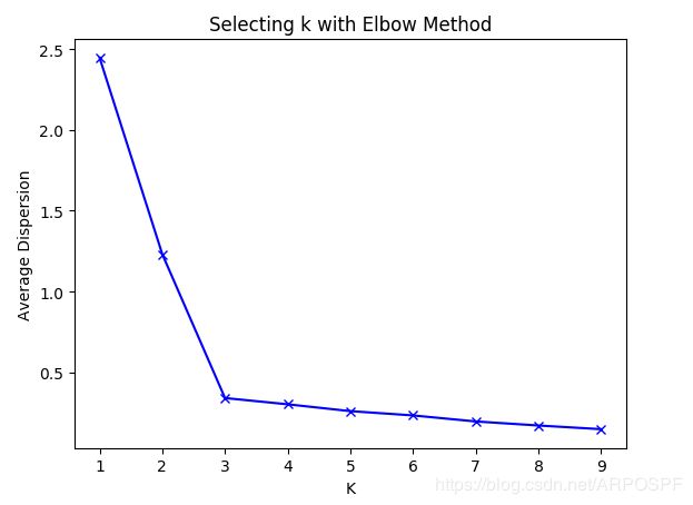
解决办法是：可以通过执行多次K-means算法来挑选性能表现更好的初始中心点；或者是使用一种“肘部”观察法用于粗略地预估相对合理的类簇个数。因为K-means模型最终期望所有数据点到其所属的类簇距离的平方和趋于稳定，所以可以通过观察这个数值随着K的走势来找出最佳的类簇数量。理想情况下，这个折线在不断下降并且趋于平缓的过程中会有斜率的拐点，同时意味着从这个拐点对应的K值开始，类簇中心的增加不会过于破坏数据聚类的结构。

#!/usr/bin/env python
# -*- coding: utf-8 -*-
"""
@File  : BestK.py
@Author: Xinzhe.Pang
@Date  : 2019/7/23 0:09
@Desc  : 
"""
import numpy as np
from sklearn.cluster import KMeans
from scipy.spatial.distance import cdist
import matplotlib.pyplot as plt

# 使用均匀分布函数随机三个簇，每个簇周围10个数据样本
cluster1 = np.random.uniform(0.5, 1.5, (2, 10))
cluster2 = np.random.uniform(5.5, 6.5, (2, 10))
cluster3 = np.random.uniform(3.0, 4.0, (2, 10))

# 绘制30个数据样本的分布图像
X = np.hstack((cluster1, cluster2, cluster3)).T
plt.scatter(X[:, 0], X[:, 1])
plt.xlabel('x1')
plt.ylabel('x2')
plt.show()

# 测试9种不同聚类中心数量下，每种情况的聚类质量，并作图
K = range(1, 10)
meandistortions = []

for k in K:
    kmeans = KMeans(n_clusters=k)
    kmeans.fit(X)
    meandistortions.append(sum(np.min(cdist(X, kmeans.cluster_centers_, 'euclidean'), axis=1)) / X.shape[0])

plt.plot(K, meandistortions, 'bx-')
plt.xlabel('K')
plt.ylabel('Average Dispersion')
plt.title('Selecting k with Elbow Method')
plt.show()