Deep Neural Networks for Object Detection
Deep Neural Networks for Object Detection
论文介绍
1) 论文来源
Szegedy C, Toshev A, Erhan D. Deep neural networks for object detection[C]//Advances in neural information processing systems. 2013: 2553-2561.
2) 论文摘要
第一次提出使用CNN解决目标检测的问题。同时达到当时同一时期最好的效果。运行时间较慢。
3) 论文下载
http://papers.nips.cc/paper/5207-deep-neural-networks-for-object-detection.pdf
主要内容
网络结构
把alexNet的最后一层softmax classifier改为softmax classifier,改为可以输出目标box在图片上的位置。规定输出的mask N = d × d N=d\times d N=d×d。比如 400 × 400 400\times 400 400×400的图片,mask = N = 24 × 24 N=24\times 24 N=24×24, 则将图片划分为16个区域,预测值mask就应该是16维向量,其中某一维或某几维,位置上的数为1,表示有目标,其余维为0。如图1所示。
损失函数

损失函数就是l2范式,因为对于一幅图片,目标所占的像素是较少的,所以网络倾向于输出0.为了避免这种情况,增加惩罚项鼓励网络输出1.
训练过程

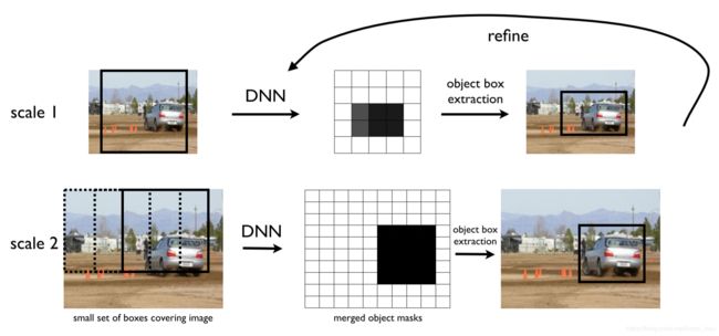
第一步,输出a binary mask of the object bounding box (and portions of the box as well)。图上的DBN应该是笔误。这样就有了目标的多个mask,如图包括整体的mask,上下左右的mask。

第二步,对每一个mask都进行更细粒度的预测。如图,先找到一个包括目标的大的box,再在这个box上提取更小的box。
这样运行多次,就可以提取到精确的object box。这是一种十分朴素的想法,但是可想而知,多次通过CNN肯定运行时间受影响。
存在的问题
论文这部分只要对三个具有挑战性的问题进行分析和解决:
第一,单个对象掩码可能不足以消除彼此相邻的对象的歧义。
1) First, a single object mask might not be sufficient to disambiguate objects which are placed next to each other.
第二,由于输出大小的限制,生成掩码比原始图像尺寸小得多(不足以精确定位一个对象)。
2)Second, due to the limits in the output size, we generate masks
that are much smaller than the size of the original image(would be insufficient to precisely localize an object).
第三,输入整张图片,小物体对输入神经元的影响很少,导致很难识别。
3)Finally, since we use as an input the full
image, small objects will affect very few input neurons and thus will be hard to recognize.
如何解决
第5章主要就是阐述如何解决上述的问题:
5 基于DNN生成掩码的精确目标定位
5 Precise Object Localization via DNN-generated Masks
5.1 用于稳健本地化的多个掩码
5.1 Multiple Masks for Robust Localization
为了处理多个生成对象,我们生成不是一个而是几个掩码,每个掩码代表完整对象或其中的一部分。由于我们的最终目标是生成一个边界框,我们使用一个网络预测对象框掩码和四个额外的网络来预测框的四个部分:底部,顶部,左半部和右半部,全部用 m h m^h mh表示,h∈{全部,下,上,左,右}。这五个预测虽然过于完整,但有助于减少不确定性并处理一些掩码中的错误。此外,如果相同类型的两个对象彼此相邻放置,则所产生的五个掩码中的至少两个将不具有合并的对象,这将允许消除它们的歧义。这将使得能够检测多个对象。
比如说一左一右两个对象,全部的掩码输出可能是一样的,但是左右掩码肯定不一样。
To deal with multiple touching objects, we generate not one but several masks, each representing either the full object or part of it. Since our end goal is to produce a bounding box, we use one network to predict the object box mask and four additional networks to predict four halves of the box: bottom, top, left and right halves, all denoted by m h m^h mh, h ∈ {full, bottom, top, left, right}. These five predictions are over-complete but help reduce uncertainty and deal with mistakes in some of the masks. Further, if two objects of the same type are placed next to each other, then at least two of the produced five masks would not have the objects merged which would allow to disambiguate them.This would enable the detection of multiple objects.
在训练时,我们需要将对象框转换为这五个掩码。由于掩码可能比原始图像小得多,我们需要将实况掩码缩小到网络输出的大小。用 T ( i , j ) T(i,j) T(i,j)表示图像中的矩形,其中对象的存在由网络的输出 ( i , j ) (i,j) (i,j)预测。此矩形的左上角位于 ( d 1 d ( i − 1 ) , d 2 d ( j − 1 ) ) (\frac {d_1}{d}(i-1),\frac {d_2}{d}(j-1)) (dd1(i−1),dd2(j−1))且大小为 d 1 d × d 1 d \frac{d_1}{d}\times\frac{d_1}{d} dd1×dd1,其中 d d d是输出掩码的大小, d 1 , d 2 d_1,d_2 d1,d2是图像的高度和宽度。在训练期间,我们指定预测值 m ( i , j ) m(i,j) m(i,j)为 T ( i , j ) T(i,j) T(i,j)由 b b ( h ) bb(h) bb(h)覆盖的部分:
At training time, we need to convert the object box to these five masks. Since the masks can be much smaller than the original image, we need to downsize the ground truth mask to the size of the network output. Denote by T ( i , j ) T(i, j) T(i,j) the rectangle in the image for which the presence of an object is predicted by output ( i , j ) (i, j) (i,j) of the network. This rectangle has upper left corner at ( d 1 d ( i − 1 ) , d 2 d ( j − 1 ) ) (\frac{d_1}{d}(i-1),\frac{d_2}{d}(j-1)) (dd1(i−1),dd2(j−1)) and has size d 1 d × d 1 d \frac{d_1}{d}\times\frac{d_1}{d} dd1×dd1,where d d d is the size of the output mask and d 1 , d 2 d_1, d_2 d1,d2 the height and width of image. During training we assign as value m ( i , j ) m(i, j) m(i,j) to be predicted as portion of T ( i , j ) T(i, j) T(i,j) being covered by box b b ( h ) bb(h) bb(h) :

其中bb(full)对应于实况对象框。 而h的其余值,bb(h)对应于原始框的四个半个的部分。
where bb(full) corresponds to the ground truth object box. For the remaining values of h, bb(h) corresponds to the four halves of the original box.
在这一点上, 应该注意的是, 人们可以为所有掩码训练一个网络, 在这个网络中, 输出层将生成所有五个掩码。这将是可伸缩的。这样, 五个本地化器将共享大部分网络层, 从而共享特征。 这似乎很自然, 因为它们处理的是同一对象。更积极的方法–对许多不同的类别使用相同的定位器–似乎也是可行的。
At this point, it should be noted that one could train one network for all masks where the output layer would generate all five of them. This would enable scalability. In this way, the five localizers would share most of the layers and thus would share features, which seems natural since they are dealing with the same object. An even more aggressive approach — using the same localizer for a lot of distinct classes – seems also workable.
5.2 输出的对象本地化
5.2 Object Localization from DNN Output
为了完成检测过程, 我们需要为每个图像估计一组边界框。虽然输出分辨率小于输入图像, 但我们将二进制掩码恢复为输入图像中的分辨率。目标是估计边界盒 bb= (i, j, k, l) ,参数由输出掩码坐标的左上角 (i, j) 和右下角 (k, l) 确定。
In order to complete the detection process, we need to estimate a set of bounding boxes for each image. Although the output resolution is smaller than the input image, we rescale the binary masks to the resolution as the input image. The goal is to estimate bounding boxes bb = (i, j, k, l) parametrized by their upper-left corner (i, j) and lower-right corner (k, l) in output mask coordinates.
为此, 我们使用分数 S 表示每个边界框 bb 与掩码的协议, 并推断得分最高的框。一个自然的协议是测量边界箱的哪一部分被掩码覆盖:
To do this, we use a score S expressing an agreement of each bounding box bb with the masks and infer the boxes with highest scores. A natural agreement would be to measure what portion of the bounding box is covered by the mask:
我们在 (i, j) 索引的所有网络输出上求和, 并用 m = DNN (x) 表示网络的输出。如果我们将上述分数扩展到所有五种掩码类型, 则最终分数为:
where we sum over all network outputs indexed by (i, j) and denote by m = DNN(x) the output of the network. If we expand the above score over all five mask types, then final score reads:
其中half = {full,bottom,top,left,left}索引整个框及其四个部分。 对于h,表示部分中的一个, h ˉ \bar h hˉ表示h的相反的部分,例如 顶部掩码应该被顶部掩码很好地覆盖,而不是底部掩码。 对于h = full,我们用 h ˉ \bar h hˉ表示bb周围的矩形区域,如果完整掩码延伸到bb之外,则其得分将受到惩罚。 在上述总和中,如果与所有五个掩码一致,则框的分数将是大的。
where halves = {full, bottom, top, left, left} index the full box and its four halves. For h denoting one of the halves h ˉ \bar h hˉ denotes the opposite half of h, e.g. a top mask should be well covered by a top mask and not at all by the bottom one. For h = full, we denote by h ˉ \bar h hˉ a rectangular region around bb whose score will penalize if the full masks extend outside bb. In the above summation, the score for a box would be large if it is consistent with all five masks.
我们使用公式(3)的得分彻底搜索可能的边界框。 我们考虑边界框的平均尺寸等于图像维度的平均值的[0.1, . . . , 0.9] 。 通过训练数据中对象框的k均值聚类估计平均图像维度和10个不同纵横比。 我们使用图像中的5个像素的步幅滑动上述90个框中的每一个。 请注意来自公式3的得分在计算了掩码m的积分图像之后,可以使用4次运算有效地计算。 确切的操作次数是5(2×#pixels + 20×#boxes),其中第一项测量积分掩码计算的复杂度,而第二项计算箱子得分计算。
We use the score from Eq. (3) to exhaustively search in the set of possible bounding boxes. We consider bounding boxes with mean dimension equal to [0.1, . . . , 0.9] of the mean image dimension and 10 different aspect ratios estimated by k-means clustering of the boxes of the objects in the training data. We slide each of the above 90 boxes using stride of 5 pixels in the image. Note that the score from Eq. (3) can be efficiently computed using 4 operations after the integral image of the mask m has been computed. The exact number of operations is 5(2 × #pixels + 20 × #boxes), where the first term measures the complexity of the integral mask computation while the second accounts for box score computation.
为了产生最终的检测集,我们执行两种类型的过滤。 第一种方法是保持盒子具有公式2定义的强分。 例如 大于0.5。 我们通过应用[14]的DNN分类器进一步修剪它们,对所关注的类进行训练,并将正分类的分类器保留在当前检测器的类中。 最后,我们应用[9]中的非最大抑制。
To produce the final set of detections we perform two types of filtering. The first is by keeping boxes with strong score as defined by Eq. (2), e.g. larger than 0.5. We further prune them by applying a DNN classifier by [14] trained on the classes of interest and retaining the positively classified ones w.r.t to the class of the current detector. Finally, we apply non-maximum suppression as in [9].
5.3 Multi-scale Refinement of DNN Localizer
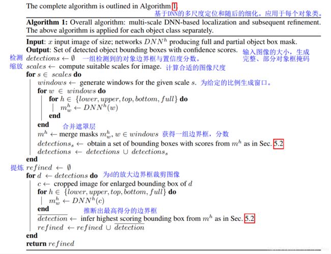
网络输出分辨率不足的问题以两种方式解决:(i)在几个尺度和几个大子窗口上应用DNN定位器; (ii)通过在顶部推断的边界框上应用DNN定位器来细化检测(参见图2)。
The issue with insufficient resolution of the network output is addressed in two ways: (i) applying the DNN localizer over several scales and a few large sub-windows; (ii) refinement of detections by applying the DNN localizer on the top inferred bounding boxes (see Fig. 2).
使用不同比例的大窗口,我们生成几个掩码并将它们合并为更高分辨率的掩码,每个比例一个。 合适的比例范围取决于图像的分辨率和定位器的感受区域的大小 - 我们希望图像被网络输出覆盖,这些输出以更高的分辨率运行,同时我们希望每个对象都是 落在至少一个窗口内,这些窗口的数量很小。
Using large windows at various scales, we produce several masks and merge them into higher resolution masks, one for each scale. The range of the suitable scales depends on the resolution of the image and the size of the receptive field of the localizer - we want the image be covered by network outputs which operate at a higher resolution, while at the same time we want each object to fall within at least one window and the number of these windows to be small.
为了实现上述目标,我们使用三个尺度:完整图像和另外两个尺度,使得给定尺度的窗口尺寸是先前尺度的窗口尺寸的一半。 我们用窗户覆盖每个比例的图像,使得这些窗口具有小的重叠 - 其面积的20%。 这些窗口的数量相对较少,并以几种比例覆盖图像。 最重要的是,最小规模的窗口允许以更高的分辨率进行定位。
To achieve the above goals, we use three scales: the full image and two other scales such that the size of the window at a given scale is half of the size of the window at the previous scale. We cover the image at each scale with windows such that these windows have a small overlap – 20% of their area. These windows are relatively small in number and cover the image at several scales. Most importantly, the windows at the smallest scale allow localization at a higher resolution.
在推理时,我们在所有窗口上应用DNN。 请注意,它与滑动窗口方法完全不同,因为我们需要评估每个图像的少量窗口,通常小于40.每个比例的生成对象掩码通过最大操作合并。 这给了我们三个图像大小的掩码,每个掩码都“看”不同大小的物体。 对于每个比例,我们应用Sec5.2中的边界框推断取得一组检测。 在我们的实施中,我们对每个比例进行了前5次检测,结果总共检测15次。
At inference time, we apply the DNN on all windows. Note that it is quite different from sliding window approaches because we need to evaluate a small number of windows per image, usually less than 40. The generated object masks at each scale are merged by maximum operation. This gives us three masks of the size of the image, each ‘looking’ at objects of different sizes. For each scale, we apply the bounding box inference from Sec. 5.2 to arrive at a set of detections. In our implementation, we took the top 5 detections per scale, resulting in a total of 15 detections.
为了进一步改善定位,我们经历了DNN回归的第二阶段,称为细化。 DNN定位器应用于由初始检测阶段定义的窗口 - 15个边界框中的每一个被放大1.2倍并应用于网络。 以更高分辨率应用定位器可显着提高检测精度。
To further improve the localization, we go through a second stage of DNN regression called refinement. The DNN localizer is applied on the windows defined by the initial detection stage – each of the 15 bounding boxes is enlarged by a factor of 1.2 and is applied to the network. Applying the localizer at higher resolution increases the precision of the detections significantly.
参考:https://blog.csdn.net/baidu88vip/article/details/81000423


