Empirical mode decomposition

[imf,residual] = emd(X)

[imf,residual,info] = emd(X)

[___] = emd(___,Name,Value)

emd(___)

Description

example

[imf,residual] = emd(X) returns intrinsic mode functions imf and residual signal residual corresponding to the empirical mode decomposition of X. Use emd to decompose and simplify complicated signals into a finite number of intrinsic mode functions required to perform Hilbert-spectral analysis.

[imf,residual,info] = emd(X) returns additional information info on IMFs and residual signal for diagnostic purposes.

[___] = emd(___,Name,Value) estimates emd with additional options specified by one or more Name,Value pair arguments.

example

emd(___) plots the original signal, IMFs, and residual signal as subplots in the same figure.

Examples

collapse all

Perform Empirical Mode Decomposition and Visualize Hilbert Spectrum of Signal

Try it in MATLAB

For this example, consider a nonstationary continuous signal composed of sinusoidal waves with a distinct change in frequency. The vibration of a jackhammer, or the sound of fireworks are examples of nonstationary continuous signals.

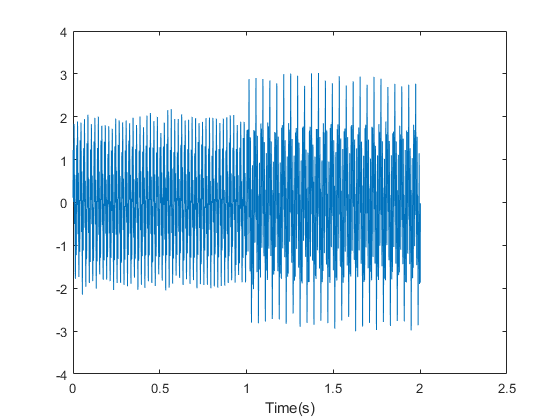
Load the nonstationary signal data with the sampling frequency fs, and visualize the mixed sinusoidal signal.

load('sinusoidalSignalExampleData.mat','X','fs');
t = (0:length(X)-1)/fs;
plot(t,X);
xlabel('Time(s)');

Observe that the mixed signal contains sinusoidal waves with different amplitude and frequency values.

In order to create the Hilbert spectrum plot, you need the IMFs of the signal. Perform empirical mode decomposition to compute the intrinsic mode functions and residuals of the signal. Since the signal is not smooth, specify 'pchip' as the Interpolation method.

[imf,residual,info] = emd(X,'Interpolation','pchip');

Current IMF  |  #Sift Iter  |  Relative Tol  |  Stop Criterion Hit  
      1      |        2     |     0.026352   |  SiftMaxRelativeTolerance
      2      |        2     |    0.0039573   |  SiftMaxRelativeTolerance
      3      |        1     |     0.024838   |  SiftMaxRelativeTolerance
      4      |        2     |      0.05929   |  SiftMaxRelativeTolerance
      5      |        2     |      0.11317   |  SiftMaxRelativeTolerance
      6      |        2     |      0.12599   |  SiftMaxRelativeTolerance
      7      |        2     |      0.13802   |  SiftMaxRelativeTolerance
      8      |        3     |      0.15937   |  SiftMaxRelativeTolerance
      9      |        2     |      0.15923   |  SiftMaxRelativeTolerance
The decomposition stopped because the number of extrema of the residual signal is less than 'MaxNumExtrema'.

The table generated in the command window indicates the number of sift iterations, the relative tolerance, and the sift stop criterion for each generated IMF. This information is also contained in info. You can hide the table by specifying Display as 0.

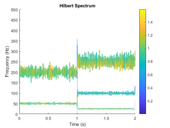
Create the Hilbert spectrum plot using the imf components obtained using empirical mode decomposition.

hht(imf,fs);

The frequency versus time plot is a sparse plot with a vertical color bar indicating the instantaneous energy at each point in the IMF. The plot represents the instantaneous frequency spectrum of each component decomposed from the original mixed signal. From the plot, three IMFs are observed with a distinct change in frequency at 1s.

Visualize Residual and Intrinsic Mode Functions of Signal

Try it in MATLAB

For this example, consider a nonstationary continuous signal composed of sinusoidal waves with a distinct change in frequency. The vibration of a jackhammer, or the sound of fireworks are examples of nonstationary continuous signals.

Load the nonstationary signal data, and visualize the mixed sinusoidal signal.

load('sinusoidalSignalExampleData.mat','X','fs');
plot(X);

Observe that the mixed signal contains sinusoidal waves with different amplitude and frequency values.

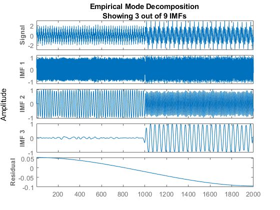
Perform empirical mode decomposition to plot the intrinsic mode functions and residual of the signal. Since the signal is not smooth, specify 'pchip' as the Interpolation method.

emd(X,'Interpolation','pchip');

Current IMF  |  #Sift Iter  |  Relative Tol  |  Stop Criterion Hit  
      1      |        2     |     0.026352   |  SiftMaxRelativeTolerance
      2      |        2     |    0.0039573   |  SiftMaxRelativeTolerance
      3      |        1     |     0.024838   |  SiftMaxRelativeTolerance
      4      |        2     |      0.05929   |  SiftMaxRelativeTolerance
      5      |        2     |      0.11317   |  SiftMaxRelativeTolerance
      6      |        2     |      0.12599   |  SiftMaxRelativeTolerance
      7      |        2     |      0.13802   |  SiftMaxRelativeTolerance
      8      |        3     |      0.15937   |  SiftMaxRelativeTolerance
      9      |        2     |      0.15923   |  SiftMaxRelativeTolerance
The decomposition stopped because the number of extrema of the residual signal is less than 'MaxNumExtrema'.

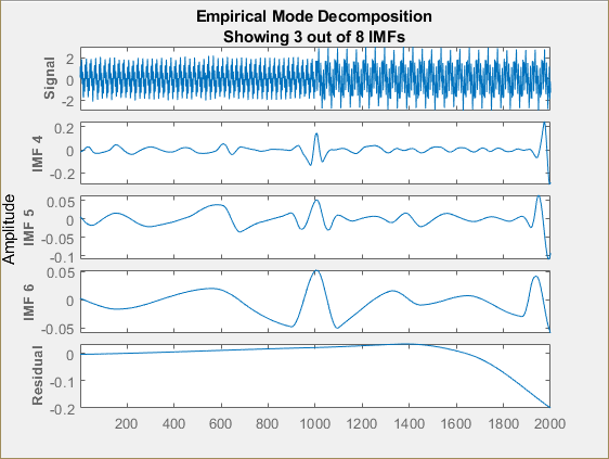
An interactive plot with the original signal, the first 3 IMFs, and the residual is generated. The table generated in the command window indicates the number of sift iterations, the relative tolerance, and the sift stop criterion for each generated IMF. You can hide the table by specifying Display as 0.

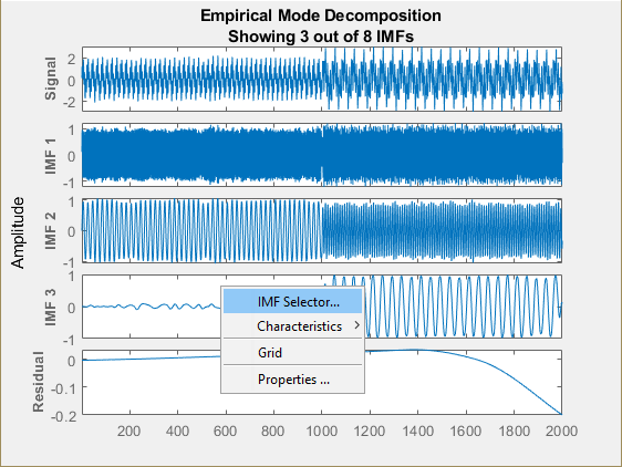
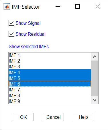
Right-click on the white space in the plot to open the IMF selector window. Use IMF selector to selectively view the generated IMFs, the original signal, and the residual.

 

 

Select the IMFs to be displayed from the list. Choose whether to display the original signal and residual on the plot.

 

 

The selected IMFs are now displayed on the plot.

 

 

Use the plot to visualize individual components decomposed from the original signal along with the residual. Note that the residual is computed for the total number of IMFs, and does not change based on the IMFs selected in the IMF selector window.

Input Arguments

collapse all

X — Uniformly sampled time-domain signal
vector | single data column timetable

Uniformly sampled time-domain signal, specified as either a vector or single data column timetable.

Name-Value Pair Arguments

Specify optional comma-separated pairs of Name,Value arguments. Name is the argument name and Value is the corresponding value. Name must appear inside quotes. You can specify several name and value pair arguments in any order as Name1,Value1,...,NameN,ValueN.

Example: 'MaxNumIMF',5

'SiftRelativeTolerance' — Cauchy type convergence criterion
0.2 (default) | positive scalar

Cauchy type convergence criterion, specified as the comma-separated pair consisting of 'SiftRelativeTolerance' and a positive scalar. SiftRelativeTolerance is one of the sifting stop criteria, that is, sifting stops when current relative tolerance is less than SiftRelativeTolerance.

'SiftMaxIterations' — Maximum number of sifting iterations
100 (default) | positive scalar integer

Maximum number of sifting iterations, specified as the comma-separated pair consisting of 'SiftMaxIterations' and a positive scalar integer. SiftMaxIterations is one of the sifting stop criteria, that is, sifting stops when the current number of iterations is larger than SiftMaxIterations.

SiftMaxIterations can be specified using only positive whole numbers.

'MaxNumIMF' — Maximum number of IMFs extracted
10 (default) | positive scalar integer

Maximum number of IMFs extracted, specified as the comma-separated pair consisting of 'MaxNumIMF' and a positive scalar integer. MaxNumIMF is one of the decomposition stop criteria, that is, decomposition stops when number of IMFs generated is equal to MaxNumIMF.

MaxNumIMF can be specified using only positive whole numbers.

'MaxNumExtrema' — Maximum number of extrema in the residual signal
1 (default) | positive scalar integer

Maximum number of extrema in the residual signal, specified as the comma-separated pair consisting of 'MaxNumExtrema' and a positive scalar integer. MaxNumExtrema is one of the decomposition stop criteria, that is, decomposition stops when number of extrema is less than MaxNumExtrema.

MaxNumExtrema can be specified using only positive whole numbers.

'MaxEnergyRatio' — Signal to residual energy ratio
20 (default) | scalar

Signal to residual energy ratio, specified as the comma-separated pair consisting of 'MaxEnergyRatio' and a scalar. MaxEnergyRatio is the ratio of the energy of the signal at the beginning of sifting and the average envelope energy.MaxEnergyRatio is one of the decomposition stop criteria, that is, decomposition stops when current energy ratio is larger than MaxEnergyRatio.

'Interpolation' — Interpolation method for envelope construction
'spline' (default) | 'pchip' | string

Interpolation method for envelope construction, specified as the comma-separated pair consisting of 'Interpolation' and either 'spline' or 'pchip'.

Specify Interpolation as:

• 'spline', if X is a smooth signal

• 'pchip', if X is a nonsmooth signal

'spline' interpolation method uses cubic spline, while 'pchip' uses piecewise cubic Hermite interpolating polynomial method.

'Display' — Toggle information display in the command window
1 (default) | 0 | scalar

Toggle information display in the command window, specified as the comma-separated pair consisting of 'Display' and either 1 or 0. The table generated in the command window indicates the number of sift iterations, the relative tolerance, and the sift stop criterion for each generated IMF. Specify Display as 1 to show the table or 0 to hide the table.

Output Arguments

collapse all

imf — Intrinsic mode function
matrix | timetable

Intrinsic mode function, returned as a matrix or timetable. imf is any function with the same number of extrema and zero crossings, whose envelope is symmetric with respect to zero. Use imf to apply Hilbert-Huang transform to perform spectral analysis on the signal.

imf is returned as:

• A matrix whose each column is an imf, when X is a vector

• A timetable, when X is a single data column timetable

 

residual — Residual of the signal
column vector | single data column timetable

Residual of the signal, returned as a column vector or a single data column timetable. residual represents the portion of the original signal X not decomposed by emd.

residual is returned as:

• A column vector, when X is a vector.

• A single data column timetable, when X is a single data column timetable.

 

info — Additional information for diagnostics
structure

Additional information for diagnostics, returned as a structure with the following fields:

• NumIMF - Number of IMFs extracted from the signal

• NumExtrema - Number of extrema in each IMF

• NumZeroCrossing - Number of zero crossings for each IMF

• NumSifting - Number of siftings performed for each IMF

• MeanEnvelopeEnergy - Energy of the mean of upper and lower envelope obtained in each IMF computation

• RelativeTolerance - Relative tolerance attained for each IMF

 

Algorithms

Empirical Mode Decomposition

emd decomposes a signal X(t) into k number of intrinsic mode functions (IMF), and residual rk(t) using the sifting process. A brief overview of the sifting process, listed in [1] and [2], is as follows:

1. Find local maxima and minima for signal X(t) to construct an upper envelope s+(t), and a lower envelope s-(t).

2. Compute mean envelope for ith iteration, mk,i(t),

   mk,i(t)=12[s+(t)+s−(t)]

3. With ck(t) = X(t) for the first iteration, subtract mean envelope from residual signal,

   ck(t)=ck(t)−mk,i(t)

   If ck(t) does not match the criteria of an IMF, steps 4 and 5 are skipped. The procedure is iterated again at step 1 with the new value of ck(t).

4. If ck(t) matches the criteria of an IMF, a new residual is computed. To update the residual signal, subtract the kth IMF from the previous residual signal,

   rk(t)=rk−1(t)−ck(t)

5. Then begin from step 1, using the residual obtained as a new signal rk(t), and store ck(t) as an intrinsic mode function.

For N intrinsic mode functions, the original signal is represented as,

X(t)=Ni=1ci(t)+rN(t)

For more information about the sifting process, see [1] and [2].

SiftRelativeTolerance

SiftRelativeTolerance is a Cauchy type stop criterion proposed in [4]. Sifting stops when current relative tolerance is less than SiftRelativeTolerance. The current relative tolerance is defined as,

RelativeTolerance≜c(t)previous−c(t)current2c(t)current2

 

MaxEnergyRatio

Energy ratio is the ratio of the energy of the signal at the beginning of sifting and the average envelope energy.[3] Decomposition stops when current energy ratio is larger than MaxEnergyRatio. For k IMFs, EnergyRatio is defined as,

EnergyRatio≜10log10(X(t)2rk(t)2)

 

References

[1] Norden E. Huang, Zheng Shen, Steven R. Long, Manli C. Wu, Hsing H. Shih, Quanan Zheng, Nai-Chyuan Yen, Chi Chao Tung, Henry H. LiuProc. R. Soc. Lond. A. "The empirical mode decomposition and the Hilbert spectrum for nonlinear and non-stationary time series analysis." Proceedings of the Royal Society of London. Series A: Mathematical, Physical and Engineering Sciences 1998. 454. 903-995. 10.1098/rspa.1998.0193.

[2] Rilling, G & Flandrin, Patrick & Gonçalves, Paulo. "On empirical mode decomposition and its algorithms." IEEE-EURASIP workshop on nonlinear signal and image processing 2003. NSIP-03. Grado, Italy. 8-11.

[3] Rato, R.T. & Ortigueira, Manuel & Batista, Arnaldo. "On the HHT, its problems, and some solutions." Mechanical Systems and Signal Processing 2008. 22. 1374-1394. 10.1016/j.ymssp.2007.11.028.

[4] Wang, Gang & Chen, Xianyao & Qiao, Fang-Li & Wu, Zhaohua & Huang, Norden. "On Intrinsic Mode Function." Advances in Adaptive Data Analysis 2010. 2. 277-293. 10.1142/S1793536910000549.

Extended Capabilities