循环神经网络RNN的前向传播与反向传播
文章目录
- 1. RNN模型
- 2. RNN的前向传播
- 3. RNN的反向传播
- 4. RNN的缺点
1. RNN模型
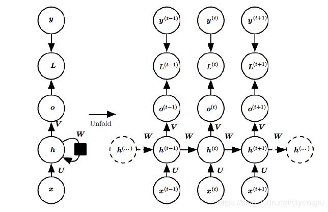
2. RNN的前向传播
对于当前的索引号 t t t,隐藏状态 h t h^t ht由 x t x^t xt和 h t − 1 h^{t-1} ht−1共同得到:
(1) h t = tanh ( U x t + W h t − 1 + b ) h^t = \tanh(Ux^t+Wh^{t-1}+b) \tag{1} ht=tanh(Uxt+Wht−1+b)(1)
其中选用了tanh作为激活函数, b b b是bias。
每次网络的输出值:
(2) o t = V h t + c o^t = Vh^t + c \tag{2} ot=Vht+c(2)
输出的预测值:
(3) a t = softmax ( o t ) = softmax ( V h t + c ) a^t = \text{softmax}(o^t) = \text{softmax}(Vh^t+c) \tag{3} at=softmax(ot)=softmax(Vht+c)(3)
使用交叉熵损失函数:
L t = − ∑ i = 1 N y i t log a i t = − log a k t L^t = -\sum_{i=1}^Ny_i^t\log a_i^t = -\log a_k^t Lt=−i=1∑Nyitlogait=−logakt
化简的结果是因为在所有的 N N N个分类中,只有 y k = 1 y_k=1 yk=1
3. RNN的反向传播
RNN的反向传播有时也叫做BPTT(back-propagation through time),所有的参数 U , W , V , b , c U, W, V, b, c U,W,V,b,c在网络的各个位置都是共享的。
成本函数:
L = ∑ t = 1 m L t L = \sum_{t=1}^mL^t L=t=1∑mLt
其中 m m m是训练集的数据量。
从《交叉熵的反向传播梯度推导(使用softmax激活函数)》一文得知,
∂ L t ∂ o t = a t − y t \frac{\partial L^t}{\partial o^t} = a^t - y^t ∂ot∂Lt=at−yt
所以
(4) ∂ L ∂ o t = ∑ t = 1 m ( a t − y t ) \frac{\partial L}{\partial o^t} = \sum_{t=1}^m(a^t - y^t) \tag{4} ∂ot∂L=t=1∑m(at−yt)(4)
参数 V , c V, c V,c的梯度可以直接计算:
{ ∂ L ∂ V = ∂ L ∂ o t ∂ o t ∂ V = ∑ t = 1 m ( a t − y t ) ( h t ) T ∂ L ∂ c = ∂ L ∂ o t ∂ o t ∂ c = ∑ t = 1 m ( a t − y t ) \left\{\begin{aligned} &\frac{\partial L}{\partial V} = \frac{\partial L}{\partial o^t} \frac{\partial o^t}{\partial V} = \sum_{t=1}^m(a^t - y^t)(h^t)^T\\ &\\ & \frac{\partial L}{\partial c} = \frac{\partial L}{\partial o^t} \frac{\partial o^t}{\partial c} = \sum_{t=1}^m(a^t - y^t) \end{aligned}\right. ⎩⎪⎪⎪⎪⎪⎪⎪⎨⎪⎪⎪⎪⎪⎪⎪⎧∂V∂L=∂ot∂L∂V∂ot=t=1∑m(at−yt)(ht)T∂c∂L=∂ot∂L∂c∂ot=t=1∑m(at−yt)
参数 W , U , b W, U, b W,U,b的梯度计算可以仿照DNN的反向传播算法,定义辅助变量,也即隐藏状态的梯度:
(5) δ t = ∂ L t ∂ h t \delta^{t} = \frac{\partial L^t}{\partial h^{t}} \tag{5} δt=∂ht∂Lt(5)
则
(6) δ t = ∂ L t ∂ o t ∂ o t ∂ h t + ∂ L t ∂ h t + 1 ∂ h t + 1 ∂ h t + ⋯ + ∂ L t ∂ h t + k ∂ h t + k ∂ h t + ⋯ = V T ( a t − y t ) + W T δ t + 1 ⊙ ( tanh ′ ( h t + 1 ) ) \begin{aligned} \delta^t &= \frac{\partial L^t}{\partial o^{t}}\frac{\partial o^t}{\partial h^{t}} + \frac{\partial L^t}{\partial h^{t+1}}\frac{\partial h^{t+1}}{\partial h^{t}} + \cdots + \frac{\partial L^t}{\partial h^{t+k}}\frac{\partial h^{t+k}}{\partial h^{t}} + \cdots\\ \\ &= V^T(a^t-y^t) + W^T\delta^{t+1}\odot(\tanh'(h^{t+1})) \tag{6} \end{aligned} δt=∂ot∂Lt∂ht∂ot+∂ht+1∂Lt∂ht∂ht+1+⋯+∂ht+k∂Lt∂ht∂ht+k+⋯=VT(at−yt)+WTδt+1⊙(tanh′(ht+1))(6)
其中只有当 k = 1 k=1 k=1,也即只有 h t + 1 h^{t+1} ht+1中才含有 h t h^t ht分量,因此式(6)中最后的扩展项中,只有 ∂ h t + 1 ∂ h t \dfrac{\partial h^{t+1}}{\partial h^{t}} ∂ht∂ht+1这一项有结果,随后的所有项,都为0。
最后一项:
(7) δ m = ∂ L m ∂ o m ∂ o m ∂ h m = V T ( a m − y m ) \delta^m = \frac{\partial L^m}{\partial o^{m}}\frac{\partial o^m}{\partial h^{m}}=V^T(a^m-y^m) \tag{7} δm=∂om∂Lm∂hm∂om=VT(am−ym)(7)
则参数 W , U , b W, U, b W,U,b的梯度可以计算如下:
(8) { ∂ L ∂ W = ∂ L ∂ h t ∂ h t ∂ W = ∑ t = 1 m δ t ⊙ ( 1 − ( h t ) 2 ) ( h t − 1 ) T ∂ L ∂ U = ∂ L ∂ h t ∂ h t ∂ U = ∑ t = 1 m δ t ⊙ ( 1 − ( h t ) 2 ) ( x t ) T ∂ L ∂ b = ∂ L ∂ h t ∂ h t ∂ b = ∑ t = 1 m δ t ⊙ ( 1 − ( h t ) 2 ) \left\{\begin{aligned} &\frac{\partial L}{\partial W} = \frac{\partial L}{\partial h^t} \frac{\partial h^t}{\partial W} = \sum_{t=1}^m \delta^t \odot (1-(h^t)^2) (h^{t-1})^T\\ &\\ &\frac{\partial L}{\partial U} = \frac{\partial L}{\partial h^t} \frac{\partial h^t}{\partial U} = \sum_{t=1}^m \delta^t \odot (1-(h^t)^2) (x^t)^T\\ &\\ & \frac{\partial L}{\partial b} = \frac{\partial L}{\partial h^t} \frac{\partial h^t}{\partial b} = \sum_{t=1}^m \delta^t\odot (1-(h^t)^2) \tag{8} \end{aligned}\right. ⎩⎪⎪⎪⎪⎪⎪⎪⎪⎪⎪⎪⎪⎪⎪⎪⎨⎪⎪⎪⎪⎪⎪⎪⎪⎪⎪⎪⎪⎪⎪⎪⎧∂W∂L=∂ht∂L∂W∂ht=t=1∑mδt⊙(1−(ht)2)(ht−1)T∂U∂L=∂ht∂L∂U∂ht=t=1∑mδt⊙(1−(ht)2)(xt)T∂b∂L=∂ht∂L∂b∂ht=t=1∑mδt⊙(1−(ht)2)(8)
其中 1 − ( h t ) 2 = tanh ′ ( h t ) 1-(h^t)^2 = \tanh'(h^t) 1−(ht)2=tanh′(ht)
4. RNN的缺点
- 前后的信息间隔变大时,RNN不能有效获得信息。对long-term dependencies 不能有效地学习。
解决方法:使用LSTM网络