AP算法实现解读

过而不悛，亡之本也。——《左传·襄公七年》

上文讲了算法数学表达式，本文就其Matlab实现以及Python实现进行代码解析，重点是理解其应用。
matlab表达式的解读是原论文已经粘贴出来的，所以直接摘抄，希望能在矩阵运算上一探究竟。
python的实现基于sklearn工具包。

Matlab 代码解读

原数学表达式为：

下面这段代码是论文中给出的示例matlab代码，但是有助于我们了解基本的实现思路。在没有考虑稀疏的相似度矩阵时：

下面进行解读：
S为一个N×N的相似度矩阵，N为数据点的数目，A和R都初始化为N×N的相似度矩阵。
第二行的作用是，主要为了防止oscillations, 该情况的发生如S是一个对称矩阵，那么a点作为b点的代表点或是相反，二者计算出来的值是一样的，那么就会引起oscillations。另外一种情况，假如我们的S是一个整数矩阵，算法可能会得到多个具有相同的网相似度的求解，算法也可能在这几个解之间oscillate。通过在S上添加机器精度级的随机噪声有助于避免这种情况。
dampening的设置也是为了防止oscillation。
算法设定的迭代次数为100次，没有early stop的步骤。但是这个显然是可以优化的。

第6行~第7行，首先计算a+s,随后第一个max求出每一行的最大值，以及通过对最大值赋值为无穷小，同时得出次大值。把行看成对应i，把列看成对应为k’。之所以这么做是用到了一个trick，就是如果k对应的是最大值，那么我们在随后第9行的赋值，使得最终使用的次大值，也就是 k′≠k 时的结果。而如果k对应的不是最大值，最终使用最大值的结果，仍然满足 k′≠k 中最大值的要求。
举个例子 ，假设我们固定i=1，这一行的s(i,k)+a(i,k)依次为：
1 5 2 3 4 这时最大值为5，4是次大值，此时我们计算方法为：

k =1	k=2	k=3	k=4	k=5
s(1,1)-5	s(1,2)-5	s(1,3)-5	s(1,4)-5	s(1,5)-5

随后对最大项下标对应位置2重新赋值为：s(1,2)-4

k =1	k=2	k=3	k=4	k=5
s(1,1)-5	s(1,2)-4	s(1,3)-5	s(1,4)-5	s(1,5)-5

就是除去该列之外的最大值。
dampenling 是为了避免数值上的oscillations,所以使用了一定的权值来进行平滑的过度。一般设定在[0.5,1)之间。

先理解公式，对于每一列，计算的是来自除去矩阵对角线的所有正值元素的和，如果不为对角线，再加上self-responsibility。
再来看第12～第14行，对角线的计算方法不同。所以矩阵中每个元素与0比较取较大值,得到仅是一个正值的矩阵，但是对角线的元素保持不变。随后对每一列求和。

假设k=1，a(i=1:5,1)= 1 2 3 4 5
(1)当i=1时，i=k 按第一个公式计算。
a(1,1)=a(1,1)+a(2,1)+a(3,1)+a(4,1)+a(5,1) - a(1,1) 而代码13行做的就是这件事。所以最终a矩阵对角线上的元素即为代码13行计算出的A矩阵的对角线上的元素，因此14行对其进行了存储。

(2)当i=2时， i≠k ，此时按公式2计算。
代码sum(Rp,1) 相当于 ∑i′≠kmax[0,r(i′,k)]+r(k,k) ，又等于
∑i′≠k，i′≠imax[0,r(i′,k)]+r(k,k)+max[r(i,k),0] ,
在第十三行减去Rp,即对应于 ∑i′≠k，i′≠imax[0,r(i′,k)]+r(k,k)+max[r(i,k),0]−max[r(i,k),0] ,
所以非对角线的元素，可以直接用第14行代码计算得出。

最后两行，是划定每个数据点所属的代表点。首先获得代表点的下标，通过 a(i,i)+r(i,i)>0 来判断，然后比较每一个数据点距离哪一个代表点距离最近，对代表点的赋值为从1到k，对数据点的赋值为代表点的标签。

[tmp c]=max(S(:,I),[],2);% 注意c是相对于选出代表集的列之后的子集的坐标
c(I)=1:K;    % 代表点的标签赋值为1到K
idx = I(c);  % 对应回原始的列下标，也就是数据点的标签

Python代码解读

下面这段代码使用了scikit-learn中的工具包，源代码如下：

from Cython.Shadow import NULL
print(__doc__)

from sklearn.cluster import AffinityPropagation
from sklearn import metrics
from sklearn.datasets.samples_generator import make_blobs

##############################################################################
# Generate sample data
centers = [[1, 1], [-1, -1], [1, -1]]
X, labels_true = make_blobs(n_samples=300, centers=centers, cluster_std=0.5,
                            random_state=0)

##############################################################################
# Compute Affinity Propagation
af = AffinityPropagation(preference=-50).fit(X)
cluster_centers_indices = af.cluster_centers_indices_
labels = af.labels_

n_clusters_ = len(cluster_centers_indices)

print('Estimated number of clusters: %d' % n_clusters_)
print("Homogeneity: %0.3f" % metrics.homogeneity_score(labels_true, labels))
print("Completeness: %0.3f" % metrics.completeness_score(labels_true, labels))
print("V-measure: %0.3f" % metrics.v_measure_score(labels_true, labels))
print("Adjusted Rand Index: %0.3f"
      % metrics.adjusted_rand_score(labels_true, labels))
print("Adjusted Mutual Information: %0.3f"
      % metrics.adjusted_mutual_info_score(labels_true, labels))
print("Silhouette Coefficient: %0.3f"
      % metrics.silhouette_score(X, labels, metric='sqeuclidean'))

##############################################################################
# Plot result
import matplotlib.pyplot as plt
from itertools import cycle

plt.close('all')
plt.figure(1)
plt.clf()

colors = cycle('bgrcmykbgrcmykbgrcmykbgrcmyk')
for k, col in zip(range(n_clusters_), colors):
    class_members = labels == k
    cluster_center = X[cluster_centers_indices[k]]
    plt.plot(X[class_members, 0], X[class_members, 1], col + '.')
    plt.plot(cluster_center[0], cluster_center[1], 'o', markerfacecolor=col,
             markeredgecolor='k', markersize=14)
    for x in X[class_members]:
        plt.plot([cluster_center[0], x[0]], [cluster_center[1], x[1]], col)

plt.title('Estimated number of clusters: %d' % n_clusters_)
plt.show()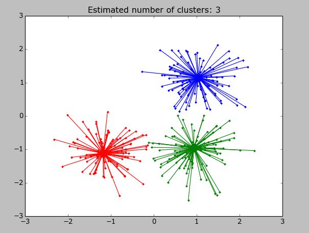

先产生待聚类的数据点，维度为300×2，其标签为300×1。
接下来看其中比较关键的部分，
在AffinityPropagtion函数中，首先检查输入的数据格式，以前的版本输入的是欧式相似度矩阵，而现在最新的版本输入格式为原始数据，或者用户自定义的相似度矩阵。

    if X.shape[0] == X.shape[1] and not self._pairwise:
        warnings.warn("The API of AffinityPropagation has changed."
                      "Now ``fit`` constructs an affinity matrix from the"
                      " data. To use a custom affinity matrix, set "
                      "``affinity=precomputed``.")
    if self.affinity is "precomputed":
        self.affinity_matrix_ = X
    elif self.affinity is "euclidean":
        self.affinity_matrix_ = -euclidean_distances(X, squared=True)
    else:
        raise ValueError("Affinity must be 'precomputed' or "
                         "'euclidean'. Got %s instead"
                         % str(self.affinity))

随后调用一个内部的函数：

   self.cluster_centers_indices_, self.labels_ = affinity_propagation(
            self.affinity_matrix_, self.preference, max_iter=self.max_iter,
            convergence_iter=self.convergence_iter, damping=self.damping,
            copy=self.copy, verbose=self.verbose)

下面解析这个函数，先来看它的默认参数：

    S: array [n_samples, n_samples]  #相似度矩阵
        Matrix of similarities between points

    preference: array [n_samples,] or float, optional, default: None
        Preferences for each point - points with larger values of
        preferences are more likely to be chosen as exemplars. The number of
        exemplars, i.e. of clusters, is influenced by the input preferences
        value. If the preferences are not passed as arguments, they will be
        set to the median of the input similarities (resulting in a moderate
        number of clusters). For a smaller amount of clusters, this can be set
        to the minimum value of the similarities.

    convergence_iter: int, optional, default: 15
        Number of iterations with no change in the number
        of estimated clusters that stops the convergence.

    max_iter: int, optional, default: 200
        Maximum number of iterations

    damping: float, optional, default: 0.5
        Damping factor between 0.5 and 1.

    copy: boolean, optional, default: True
        If copy is False, the affinity matrix is modified inplace by the
        algorithm, for memory efficiency

    verbose: boolean, optional, default: False  # 详细显示
        The verbosity level

对A和R矩阵进行初始化，把preference放在对角线位置上，这其实就是 s(k,k) ，作为用户的输入值，代表着在初始阶段一个数据点有适合作为代表点。

    # Place preference on the diagonal of S
    S.flat[::(n_samples + 1)] = preference

    A = np.zeros((n_samples, n_samples))
    R = np.zeros((n_samples, n_samples))  # Initialize messages

    # Remove degeneracies
    S += ((np.finfo(np.double).eps * S + np.finfo(np.double).tiny * 100) *
          random_state.randn(n_samples, n_samples))

在S矩阵上添加少量随机噪声，上文已经解释过了。噪声的规模非常小，对最后的结果不会有影响。

   # Execute parallel affinity propagation updates
    e = np.zeros((n_samples, convergence_iter))

    ind = np.arange(n_samples)#ind一开始

    for it in range(max_iter):
        # Compute responsibilities
        Rold = R.copy()
        AS = A + S

        I = np.argmax(AS, axis=1)# 每一行的最大值的列坐标
        Y = AS[np.arange(n_samples), I]  # np.max(AS, axis=1)#每一行的最大值提取出来

        AS[ind, I[ind]] = - np.finfo(np.double).max # 把每一行最大值赋值为数值域的最小值

        Y2 = np.max(AS, axis=1) # 再次求每一行的最大值，这是另一种写法
        R = S - Y[:, np.newaxis] # S每一行各个数字都减去AS这一行的最大值

        R[ind, I[ind]] = S[ind, I[ind]] - Y2[ind]# 但是最大值的所在列，要减去这一行的次大值

        R = (1 - damping) * R + damping * Rold  # Damping

        # Compute availabilities
        Aold = A
        Rp = np.maximum(R, 0)
        Rp.flat[::n_samples + 1] = R.flat[::n_samples + 1]#存储对角线值

        A = np.sum(Rp, axis=0)[np.newaxis, :] - Rp #相当于matlab代码第十三行

        dA = np.diag(A)
        A = np.minimum(A, 0)

        A.flat[::n_samples + 1] = dA

        A = (1 - damping) * A + damping * Aold  # Damping #加权平均

        # Check for convergence
        E = (np.diag(A) + np.diag(R)) > 0 #对角线的元素中A+R
        e[:, it % convergence_iter] = E #记录messages decision为一列
        K = np.sum(E, axis=0)

        if it >= convergence_iter:
            se = np.sum(e, axis=1)
            unconverged = (np.sum((se == convergence_iter) + (se == 0))
                           != n_samples)#对每一列求和，如果没有改变，那么全都是1或全是0，求和后为convergence_iter或者为0，再统计是不是所有的样本都满足这个条件
            if (not unconverged and (K > 0)) or (it == max_iter):
                if verbose:
                    print("Converged after %d iterations." % it)
                break
    else:
        if verbose:
            print("Did not converge")

随后退出迭代，得到最后结果：

  I = np.where(np.diag(A + R) > 0)[0]# 表示代表点的index
  K = I.size  # Identify exemplars #有多少个代表点

  if K > 0:
     c = np.argmax(S[:, I], axis=1)#代表使得a(i,k)+r(i,k)最大的k
     c[I] = np.arange(K)  # Identify clusters
     # Refine the final set of exemplars and clusters and return results
     # 这几步是上面算法中没有提到的，对于计算出的exemplar的修订
     for k in range(K):
         ii = np.where(c == k)[0]#标签为k的数据点下标
         #注意newaxis用法例如ii[:,np.newaxis]维度为(114,1),而ii为(114，）
         #假设ii为1 4 6选择了同一个代表点，结合起来就是
         # (1,1) (1,4) (1,6)
         # (4,1) (4,4) (4,6)
         # (6,1) (6,4) (6,6)
         # 这里先对每一列求和，再输出最大值的相对于ii的下标
         # 我的理解是相当于再发动了一次选举，在选同一个代表点的数据中选出和别的代表点相似度最高的新代表点
         j = np.argmax(np.sum(S[ii[:, np.newaxis], ii], axis=0))
         I[k] = ii[j]

     c = np.argmax(S[:, I], axis=1) #同matlab代码19行
     c[I] = np.arange(K)#同matlab代码19行
     labels = I[c]#同matlab代码19行
     # Reduce labels to a sorted, gapless, list
     cluster_centers_indices = np.unique(labels)
     labels = np.searchsorted(cluster_centers_indices, labels)#之前得到的是以绝对列下标命名，比如160 252 272，将数据点的标签对应改为0 1 2，
  else:
     labels = np.empty((n_samples, 1))
     cluster_centers_indices = None
     labels.fill(np.nan)
  return cluster_centers_indices, labels