《机器学习》k近邻(KNN)
本文主要讲述机器学习监督学习之KNN最近邻分类算法,希望通过概念的介绍,公式的推理以及案例分析,让你更了解K近邻算法。
内容包括:
1.k近邻基础知识
2.k近邻算法的公式推导
3.纯Python实现k近邻算法
4.k近邻算法的案例分析
1.k近邻基础知识
K近邻是由Cover和Hart在1968年提出,其思想就是“你与你的邻居很相似”。所以对于分类来说,找到K个最近的邻居,用投票法找出最多数的类别,然后将数据点预测为该类别。同理,回归的话输出最近的K个样本的平均值作为预测值。
举例讲解K近邻法,现在有一个红色圆圈,为待分类点,判断红色圆点属于三角形还是正方形类别,采用K近邻分类的思想为:

1.当K=3时,图中第一个圈包含了3个图形,其中三角形1个,正方形2个,该圆的则分类结果为正方形类标。
2.当K=5时,第二个圈中包含了5个图形,三角形3个,正方形2个,则以3:2的投票结果预测圆为三角形类标。
总之,设置不同的K值,可能预测得到不同的结果。k 值的大小对分类结果有着重大的影响。当选择的 k 值较小,模型预测结果会对实例点非常敏感,分类器抗噪能力较差,因而容易产生过拟合。
如果选择较大的 k 值,就相当于在用较大邻域中的训练实例进行预测,会增加分类误差会产生一定程度的欠拟合。为了选择合适的k值。
一般采用交叉验证的方式来选择合适的 k 值,经验规则:K一般低于训练样本数的平方根。
2.k近邻算法的公式推导
(1)距离度量
距离的度量用在 k 近邻中我们也可以称之为相似性度量,即特征空间中两个实例点相似程度的反映。在 k 近邻算法中常用的距离度量方式是欧式距离,也即 L2 距离,L2 距离计算公式如下:
最常用的是欧式距离:

曼哈顿距离:
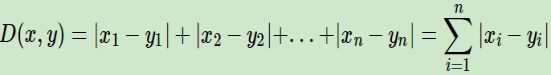
通用的闵可夫斯基距离:

3.纯Python实现k近邻算法
第一步:划分测试集与训练集
第二步:计算欧氏距离
第三步:用交叉验证法计算最优K
第四步:K近邻做预测
import pandas as pd
import numpy as np
data = pd.read_csv("balance-scale.csv",sep =",",header=None)
import numpy as np
from collections import Counter
import random
import matplotlib.pyplot as plt
from sklearn import datasets
from sklearn.datasets import load_iris
from sklearn.utils import shuffle
#设置绘图参数
plt.rcParams['figure.figsize'] = (10.0, 8.0)
plt.rcParams['image.interpolation'] = 'nearest'
plt.rcParams['image.cmap'] = 'gray'
#定义K近邻类
class KNearestNeighbor(object):
    def __init__(self):
        pass

    def train(self, X, y):
        self.X_train = X
        self.y_train = y
    #计算欧式距离
    def compute_distances(self, X):
        num_test = X.shape[0]
        num_train = self.X_train.shape[0]
        dists = np.zeros((num_test, num_train))
        M = np.dot(X, self.X_train.T)
        te = np.square(X).sum(axis=1)
        tr = np.square(self.X_train).sum(axis=1)
        dists = np.sqrt(-2 * M + tr + np.matrix(te).T)
        return dists
    #定义分类决策规则,默认K值为1 , np.argsort是提取距离从小到大排列的索引,将标签转换为以为数组,取前k个
    def predict_labels(self, dists, k=1):
        num_test = dists.shape[0]
        y_pred = np.zeros(num_test)
        for i in range(num_test):
            closest_y = []
            labels = self.y_train[np.argsort(dists[i, :])].flatten()
            closest_y = labels[0:k]
            c = Counter(closest_y)
            y_pred[i] = c.most_common(1)[0][0]
        return y_pred
    #进行5择交叉验证来选择最优的K值
    def cross_validation(self, X_train, y_train):
        num_folds = 5
        k_choices = [1, 3, 5, 8, 10, 12, 15, 20, 50, 100]

        X_train_folds = []
        y_train_folds = []

        X_train_folds = np.array_split(X_train, num_folds)
        y_train_folds = np.array_split(y_train, num_folds)

        k_to_accuracies = {}
        for k in k_choices:
            for fold in range(num_folds):
                 # 对传入的训练集单独划出一个验证集作为测试集fold=1,k=3
                validation_X_test = X_train_folds[fold]
                validation_y_test = y_train_folds[fold]
                temp_X_train = np.concatenate(X_train_folds[:fold] + X_train_folds[fold + 1:])
                temp_y_train = np.concatenate(y_train_folds[:fold] + y_train_folds[fold + 1:])

                # 计算距离
                self.train(temp_X_train, temp_y_train )

                temp_dists = self.compute_distances(validation_X_test)
                temp_y_test_pred = self.predict_labels(temp_dists, k=k)
                temp_y_test_pred = temp_y_test_pred.reshape((-1, 1))                #Checking accuracies
                # 查看分类准确率
                num_correct = np.sum(temp_y_test_pred == validation_y_test)
                num_test = validation_X_test.shape[0]
                accuracy = float(num_correct) / num_test
                k_to_accuracies[k] = k_to_accuracies.get(k,[]) + [accuracy]        # Print out the computed accuracies
        # 打印不同 k 值不同折数下的分类准确率
        for k in sorted(k_to_accuracies):
            for accuracy in k_to_accuracies[k]:
                print('k = %d, accuracy = %f' % (k, accuracy))

        accuracies_mean = np.array([np.mean(v) for k,v in sorted(k_to_accuracies.items())])
        best_k = k_choices[np.argmax(accuracies_mean)]
        print('最佳k值为{}'.format(best_k))

        return best_k
    # 划分训练集与测试集,先用shuffle() 将序列的所有元素随机排序。取数据集的0.7为训练集,数据集的0.3为测试集
    def create_train_test(self,data_x,data_y):
        X, y = shuffle(data_x,data_y,random_state=13)
        #用astype将X数组转换数据类型
        X = X.astype(np.float32)
        #将y变换为一列数组
        y = y.reshape((-1,1))
        offset = int(X.shape[0] * 0.7)
        #取数据集的前百分之70为训练集
        X_train, y_train = X[:offset], y[:offset]
        #取后百分之30%为测试集
        X_test, y_test = X[offset:], y[offset:]
        y_train = y_train.reshape((-1,1))
        y_test = y_test.reshape((-1,1))
        return X_train, y_train, X_test, y_test
if __name__ == '__main__':
    knn_classifier = KNearestNeighbor()
    iris=load_iris()
    X_train, y_train, X_test, y_test = knn_classifier.create_train_test(iris.data, iris.target)
    best_k = knn_classifier.cross_validation(X_train, y_train)
    X=X_test
    dists = knn_classifier.compute_distances(X_test)
    y_test_pred = knn_classifier.predict_labels(dists, k=best_k)
    y_test_pred = y_test_pred.reshape((-1, 1))
    num_correct = np.sum(y_test_pred == y_test)
    accuracy = float(num_correct) / X_test.shape[0]
    print('Got %d / %d correct => accuracy: %f' % (num_correct, X_test.shape[0], accuracy))
4. K近邻分析平衡秤数据集
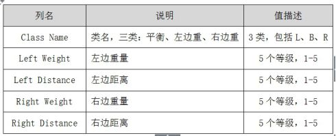
数据集主要来自于平衡秤的重量和距离相关数据,共625个样本,4个特征。这个数据集被生成来模拟心理实验结果。每个例子被分类为具有平衡尺度尖端向右,向左倾斜或平衡。属性是左侧重量,左侧距离,右侧重量和右侧距离。找到类的正确方法是(左距离左权重)和(右距离右权重)中的较大者。如果他们平等,就是平衡的。属性如下表所示:
if __name__ == '__main__':
    knn_classifier = KNearestNeighbor()
    data = pd.read_csv("balance-scale.csv",sep =",",header=None)
    X_train, y_train, X_test, y_test = knn_classifier.create_train_test(data.iloc[:,1:],data.iloc[:,0:1])
    best_k = knn_classifier.cross_validation(X_train, y_train)
    dists = knn_classifier.compute_distances(X_test)
    y_test_pred = knn_classifier.predict_labels(dists, k=best_k)
    y_test_pred = y_test_pred.reshape((-1, 1))
    num_correct = np.sum(y_test_pred == y_test)
    accuracy = float(num_correct) / X_test.shape[0]
    print('Got %d / %d correct => accuracy: %f' % (num_correct, X_test.shape[0], accuracy))
    data = pd.read_csv("balance-scale.csv",sep =",",header=None)
    x_min,x_max=X_test.iloc[:,0].min()-0.5,X_test.iloc[:,0].max()+0.5
    y_min,y_max=X_test.iloc[:,1].min()-0.5,X_test.iloc[:,1].max()+0.5

    cmap_light=ListedColormap(['#AAAAFF','#AAFFAA','#FFAAAA'])
    cmap_bold = ListedColormap(['#FF0000', '#00FF00', '#0000FF'])
    h=0.5
    xx,yy=np.meshgrid(np.arange(x_min,x_max,h),np.arange(y_min,y_max,h))

    #knn=KNeighborsClassifier()
    #knn.fit(x,y)
    z = knn_classifier.predict_labels(dists, k=best_k)[:100]
    z=z.reshape(xx.shape)
    plt.figure()
    y_test=y_test.reshape((-1, 1))
    plt.pcolormesh(xx,yy,z,cmap=cmap_light)
    a=np.array(X_test.iloc[:,1]).reshape((-1, 1))
    b=np.array(X_test.iloc[:,0]).reshape((-1, 1))
    plt.scatter(b, a, c=y_test, cmap=cmap_bold, s=50)
    plt.title('基于balance-scale数据集的k近邻')
    plt.xlim(xx.min(),xx.max())
    plt.ylim(yy.min(),yy.max())
    plt.show()
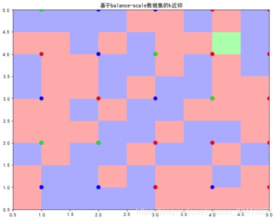
可以看到整个区域划分为三种颜色,绿色区域、红色区域和蓝色区域。同时包括散点图分布,对应数据的类标,包括绿色、蓝色和红色的点。可以发现,相同颜色的点主要集中于该颜色区域,部分蓝色点划分至红色区域或绿色点划分至蓝色区域,则表示预测结果与实际结果不一致。
参考文档