caffe2 学习笔记04-训练网络并进行预测

caffe2 学习笔记04-训练网络并进行预测

1. 前言

基于caffe2 示例中的MNIST网络(原文(链接在此))，改进用于识别车牌31个汉字，训练用的数据来自上一篇[caffe2 学习笔记03-从图片如何到mdb数据集

2. 理论准备

1. 公式：
   学习速率公式，原文公式（疑有误？）：t是迭代次数
   
   learning rate=base_lr∗tgamma
   
   我认为应该是：
   
   learning rate=base_lr∗gammat
   
   这样，学习速率才会逐渐下降，原文中给出的公式可能有误；

原文中,初始参数：

base_r=−0.1   stepsize=1   gamma=0.999

3.import库文件

%matplotlib inline
from matplotlib import pyplot
import numpy as np
import os
import shutil

import caffe2.python.predictor.predictor_exporter as pe

from caffe2.python import core, model_helper, net_drawer, workspace, visualize, brew
import time
# If you would like to see some really detailed initializations,
# you can change --caffe2_log_level=0 to --caffe2_log_level=-1
core.GlobalInit(['caffe2', '--caffe2_log_level=0'])
print("Necessities imported!")

4.准备

data_folder = "/home/hw/main-data/02_work/12_caffe2_char" #数据所在文件夹

定义若干函数：

def AddInput(model, batch_size, db, db_type):  #载入数据
    # load the data

    data_uint8, label = model.TensorProtosDBInput(
        [], ["data_uint8", "label"], batch_size=batch_size,
        db=db, db_type=db_type)

    # cast the data to float
    data = model.Cast(data_uint8, "data", to=core.DataType.FLOAT)
    # scale data from [0,255] down to [0,1]
#     data = model.Scale(data, data, scale=float(1./256))
    # don't need the gradient for the backward pass
    data = model.StopGradient(data, data)
    return data, label

def AddLeNetModel(model, data): #设置网络
    """
    This part is the standard LeNet model: from data to the softmax prediction.

    For each convolutional layer we specify dim_in - number of input channels
    and dim_out - number or output channels. Also each Conv and MaxPool layer changes the
    image size. For example, kernel of size 5 reduces each side of an image by 4.

    While when we have kernel and stride sizes equal 2 in a MaxPool layer, it divides
    each side in half.
    """
    # Image size: 28 x 28 -> 24 x 24
    conv1 = brew.conv(model, data, 'conv1', dim_in=3, dim_out=20, kernel=5)
    # Image size: 24 x 24 -> 12 x 12
    pool1 = brew.max_pool(model, conv1, 'pool1', kernel=2, stride=2)
    # Image size: 12 x 12 -> 8 x 8
    conv2 = brew.conv(model, pool1, 'conv2', dim_in=20, dim_out=100, kernel=5)
    # Image size: 8 x 8 -> 4 x 4
    pool2 = brew.max_pool(model, conv2, 'pool2', kernel=2, stride=2)
    # 50 * 4 * 4 stands for dim_out from previous layer multiplied by the image size
    fc3 = brew.fc(model, pool2, 'fc3', dim_in=100 * 4 * 4, dim_out=500)

    #fc3 = brew.relu(model, fc3, fc3)
    relu = brew.relu(model, fc3, fc3)
    pred = brew.fc(model, relu, 'pred', 500, 31)
    softmax = brew.softmax(model, pred, 'softmax')
    return softmax

def AddAccuracy(model, softmax, label): #添加精度记录
    """Adds an accuracy op to the model"""
    accuracy = brew.accuracy(model, [softmax, label], "accuracy")
    return accuracy

def AddTrainingOperators(model, softmax, label): #添加训练操作符
    """Adds training operators to the model."""
    xent = model.LabelCrossEntropy([softmax, label], 'xent')
    # compute the expected loss
    loss = model.AveragedLoss(xent, "loss")
    # track the accuracy of the model
    AddAccuracy(model, softmax, label)
    # use the average loss we just computed to add gradient operators to the model
    model.AddGradientOperators([loss])
    # do a simple stochastic gradient descent
    ITER = brew.iter(model, "iter")
    # set the learning rate schedule

    ############################### 设置学习速率 ###############################
    LR = model.LearningRate(
        ITER, "LR", base_lr=-0.0083, policy="step", stepsize=1, gamma=0.999 )   # lr = base_lr * (t ^ gamma) #学习速率的设置非常重要，下边的说明
    ############################### 设置学习速率 ###############################

    # ONE is a constant value that is used in the gradient update. We only need
    # to create it once, so it is explicitly placed in param_init_net.
    ONE = model.param_init_net.ConstantFill([], "ONE", shape=[1], value=1.0)
    # Now, for each parameter, we do the gradient updates.
    for param in model.params:
        # Note how we get the gradient of each parameter - ModelHelper keeps
        # track of that.
        param_grad = model.param_to_grad[param]
        # The update is a simple weighted sum: param = param + param_grad * LR
        model.WeightedSum([param, ONE, param_grad, LR], param)

def AddBookkeepingOperators(model): #添加记录符
    """This adds a few bookkeeping operators that we can inspect later.

    These operators do not affect the training procedure: they only collect
    statistics and prints them to file or to logs.
    """    
    # Print basically prints out the content of the blob. to_file=1 routes the
    # printed output to a file. The file is going to be stored under
    #     root_folder/[blob name]
    model.Print('accuracy', [], to_file=1)
    model.Print('loss', [], to_file=1)
    # Summarizes the parameters. Different from Print, Summarize gives some
    # statistics of the parameter, such as mean, std, min and max.
    for param in model.params:
        model.Summarize(param, [], to_file=1)
        model.Summarize(model.param_to_grad[param], [], to_file=1)
    # Now, if we really want to be verbose, we can summarize EVERY blob
    # that the model produces; it is probably not a good idea, because that
    # is going to take time - summarization do not come for free. For this
    # demo, we will only show how to summarize the parameters and their
    # gradients.

5. 初始化训练及测试网络

train_name = "train" #chn_train
test_name = "test"

arg_scope = {"order": "NCHW"}
train_model = model_helper.ModelHelper(name = train_name, arg_scope=arg_scope)

train_model.param_init_net.RunAllOnGPU()
train_model.net.RunAllOnGPU()
#------------------------------ set train mode ----------------------------
data, label = AddInput(
    train_model, batch_size=2048,  #单次batch数目，设置非常重要，下边有表述
    db=os.path.join(data_folder, train_name),
    db_type='lmdb')
print "train path: ", os.path.join(data_folder, train_name)
softmax = AddLeNetModel(train_model, data)
AddTrainingOperators(train_model, softmax, label)
AddBookkeepingOperators(train_model)

# Testing model. We will set the batch size to 100, so that the testing
# pass is 100 iterations (10,000 images in total).
# For the testing model, we need the data input part, the main LeNetModel
# part, and an accuracy part. Note that init_params is set False because
# we will be using the parameters obtained from the train model.
test_model = model_helper.ModelHelper(
    name = test_name, arg_scope=arg_scope, init_params=False)

test_model.param_init_net.RunAllOnGPU() #设置为GPU模式，用CPU运行，速度很慢
test_model.net.RunAllOnGPU()
#------------------------------ set train mode ----------------------------
#------------------------------ set test mode -----------------------------
data, label = AddInput(
    test_model, batch_size=512,
    db=os.path.join(data_folder, test_name),
    db_type='lmdb')
print "test path: ", os.path.join(data_folder, test_name)
softmax = AddLeNetModel(test_model, data)
AddAccuracy(test_model, softmax, label)

# Deployment model. We simply need the main LeNetModel part.
deploy_model = model_helper.ModelHelper(
    name="mnist_deploy", arg_scope=arg_scope, init_params=False)
AddLeNetModel(deploy_model, "data")
# You may wonder what happens with the param_init_net part of the deploy_model.
# No, we will not use them, since during deployment time we will not randomly
# initialize the parameters, but load the parameters from the db.
#------------------------------ set test mode -----------------------------

6. 训练

before = time.time()
localtime = time.localtime(before)
print("start at : ", time.asctime(localtime))
# The parameter initialization network only needs to be run once.
workspace.RunNetOnce(train_model.param_init_net)
# creating the network
workspace.CreateNet(train_model.net, overwrite=True)
# set the number of iterations and track the accuracy & loss
total_iters = 10000
accuracy = np.zeros(total_iters)
loss = np.zeros(total_iters)
# Now, we will manually run the network for 200 iterations.


for i in range(total_iters):
#     print("iter: ",i)
    workspace.RunNet(train_model.net)

    accuracy[i] = workspace.FetchBlob('accuracy')
    loss[i] = workspace.FetchBlob('loss')

after = time.time()
# After the execution is done, let's plot the values.

print("time in seconds: ", after - before)
print("time in minutes: ", (after - before)/60)
localtime = time.localtime(after)
print("end at : ", time.asctime(localtime))
pyplot.plot(loss, 'b')
pyplot.plot(accuracy, 'r')
pyplot.legend(('Loss', 'Accuracy'), loc='upper right')

开始训练：

before = time.time()
localtime = time.localtime(before)
print("start at : ", time.asctime(localtime))
# The parameter initialization network only needs to be run once.
workspace.RunNetOnce(train_model.param_init_net)
# creating the network
workspace.CreateNet(train_model.net, overwrite=True)
# set the number of iterations and track the accuracy & loss
total_iters = 10000
accuracy = np.zeros(total_iters)
loss = np.zeros(total_iters)
# Now, we will manually run the network for 200 iterations.


for i in range(total_iters):
#     print("iter: ",i)
    workspace.RunNet(train_model.net)

    accuracy[i] = workspace.FetchBlob('accuracy')
    loss[i] = workspace.FetchBlob('loss')

after = time.time()
# After the execution is done, let's plot the values.

print("time in seconds: ", after - before)
print("time in minutes: ", (after - before)/60)
localtime = time.localtime(after)
print("end at : ", time.asctime(localtime))
pyplot.plot(loss, 'b')
pyplot.plot(accuracy, 'r')
pyplot.legend(('Loss', 'Accuracy'), loc='upper right')

输出：

('start at : ', 'Thu Aug 31 13:59:06 2017')
('time in seconds: ', 2490.3361990451813)
('time in minutes: ', 41.50560331741969)
('end at : ', 'Thu Aug 31 14:40:36 2017')

正常训练结果如下：

尽管有波动，但是能够看出loss值在逐渐降低，accuracy在逐渐向1贴近，模型有收敛的趋势

不正常的训练结果：

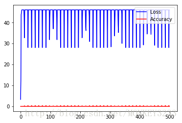
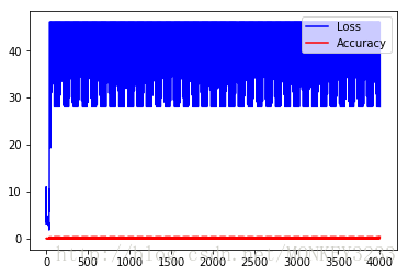
可见，loss并未降低，而是增大，并且呈现周期性，accuracy看不清，但是肯定不是趋近于1的

经过分析，发现 learning rate，batch_size，总训练数据量training set存在如下关系时，训练曲线是较为正常的

batch_sizetraining set∗1learning rate=3.3

分析结果：当batch size过小，同时learning rate相对过大时，会让模型进入局部陷阱中震荡，无法跳出局部最优区域，从而呈现出上边第3~4图现象

7. 测试

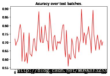
利用test数据集进行测试，当然，实际应该用validation数据集选择模型，然后用test数据集测试最终选择好的模型结果；
测试代码如下：

before = time.time()
localtime = time.localtime(before)
print("start at : ", time.asctime(localtime))

workspace.RunNetOnce(test_model.param_init_net)
workspace.CreateNet(test_model.net, overwrite=True)
test_accuracy = np.zeros(100)
for i in range(100):
    workspace.RunNet(test_model.net.Proto().name)
    test_accuracy[i] = workspace.FetchBlob('accuracy')
# After the execution is done, let's plot the values.
pyplot.plot(test_accuracy, 'r')
pyplot.title('Acuracy over test batches.')
print('test_accuracy: %f' % test_accuracy.mean())

after = time.time()

print("time in seconds: ", after - before)
print("time in minutes: ", (after - before)/60)
localtime = time.localtime(after)
print("end at : ", time.asctime(localtime))

输出结果：

('start at : ', 'Thu Aug 31 13:55:28 2017')
test_accuracy: 0.708770
('time in seconds: ', 2.4325649738311768)
('time in minutes: ', 0.040542749563852946)
('end at : ', 'Thu Aug 31 13:55:30 2017')

8. 存储model

# construct the model to be exported
# the inputs/outputs of the model are manually specified.
pe_meta = pe.PredictorExportMeta(
    predict_net=deploy_model.net.Proto(),
    parameters=[str(b) for b in deploy_model.params],
    inputs=["data"],
    outputs=["softmax"],
)

# save the model to a file. Use minidb as the file format
pe.save_to_db("minidb", os.path.join(data_folder, "tmp_100.minidb"), pe_meta)
print("The deploy model is saved to: " + data_folder + "/tmp_100.minidb")