TensorFlow实战2：实现多项式回归

上篇文章中我们讲解了单变量线性回归的例子，对于非线性的数据分布，用单变量线性回归拟合程度一般，我们来试试多项式回归。

前面的步骤还是和上篇一样，后面会添加多个变量来对数据进行拟合。

1、数据准备
实际的数据大家可以通过pandas等package读入，也可以使用自带的Boston House Price数据集，这里为了简单，我们自己手造一点数据集。

%matplotlib inline
import numpy as np
import tensorflow as tf
import matplotlib.pyplot as plt
plt.rcParams["figure.figsize"] = (14,8)

n_observations = 100
xs = np.linspace(-3, 3, n_observations)
ys = np.sin(xs) + np.random.uniform(-0.5, 0.5, n_observations)
plt.scatter(xs, ys)
plt.show()

2.准备好placeholder,开好容器来装数据

X = tf.placeholder(tf.float32, name='X')
Y = tf.placeholder(tf.float32, name='Y')

3.初始化参数/权重

W = tf.Variable(tf.random_normal([1]),name = 'weight')
b = tf.Variable(tf.random_normal([1]),name = 'bias')

4.计算预测结果

Y_pred = tf.add(tf.multiply(X,W), b)

#添加高次项
W_2 = tf.Variable(tf.random_normal([1]),name = 'weight_2')
y_pred = tf.add(tf.multiply(tf.pow(X,2),W_2), Y_pred)
W_3 = tf.Variable(tf.random_normal([1]),name = 'weight_3')
Y_pred = tf.add(tf.multiply(tf.pow(X,3),W_3), Y_pred)
# W_4 = tf.Variable(tf.random_normal([1]),name = 'weight_4')
# Y_pred = tf.add(tf.multiply(tf.pow(X,4),W_4), Y_pred)

5.计算损失函数值

sample_num = xs.shape[0]   #取出xs的个数，这里是100个
loss = tf.reduce_sum(tf.pow(Y_pred - Y,2))/sample_num     #向量对应的点相减之后，求平方和，在除以点的个数

6.初始化optimizer

learning_rate = 0.01
optimizer = tf.train.GradientDescentOptimizer(learning_rate).minimize(loss)

7.指定迭代次数，并在session里执行graph

n_samples = xs.shape[0]
init = tf.global_variables_initializer()
with tf.Session() as sess:
    #初始化所有变量
    sess.run(init)

    #将搜集的变量写入事件文件，提供给Tensorboard使用
    writer = tf.summary.FileWriter('./graphs/polynomial_reg',sess.graph)

    #训练模型
    for i in range(1000):
        total_loss = 0    #设定总共的损失初始值为0
        for x,y in zip(xs,ys):      #zip:将两个列表中的对应元素分别取一个出来，形成一个元组
            _, l = sess.run([optimizer, loss], feed_dict={X: x, Y:y}) 
            total_loss += l     #计算所有的损失值进行叠加

        if i%100 ==0:
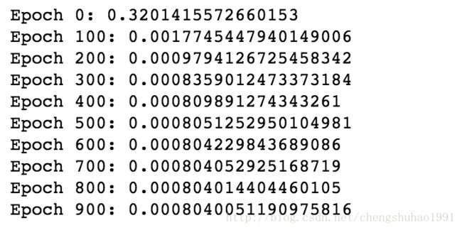
            print('Epoch {0}: {1}'.format(i, total_loss/n_samples))

    # 关闭writer
    writer.close()
    # 取出w和b的值
    W, W_2, W_3, b = sess.run([W, W_2, W_3, b])    

迭代的打印结果为下图：

打印参数

print("W:"+str(W[0]))
print("W_2:"+str(W_2[0]))
print("W_3:"+str(W_3[0]))
print("W_4:"+str(W_4[0]))
print("b:"+str(b[0]))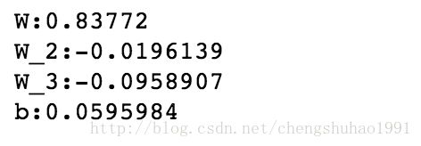

作图

plt.plot(xs, ys, 'bo', label='Real data')    #真实值的散点
plt.plot(xs, xs*W + np.power(xs,2)*W_2 + np.power(xs,3)*W_3 + b, 'r', label='Predicted data')    #预测值的拟合线条
plt.legend()     #用于显示图例  
plt.show()      #显示图

从图中可以看到，在使用了三个变量的多项式回归之后，对数据点的拟合程度达到了较高的要求，其实此处使用的三个变量就是sin()的泰勒展开函数。如果还需要更近一步的进行拟合的话，可以增加变量的个数以及阶数。