Multi-Task Learning as Multi-Objective Optimization 阅读笔记

通常multi-task learning的任务优化的是多个任务的线性组合，但这只在多个任务是不竞争的情况下是有效的。文章将multi-task learning的任务当做multi-objective optimization的问题来处理，寻找帕累托最优解。作者使用gradient-based multiobjective optimization来优化multi-objective optimization问题。但在参数量巨大和task多的情况下复杂度高，作者提出优化一个上界，并证明在现实情况下，优化这个上界可以得到帕累托最优解。

Multi-Task Learning（MTL）

假设有一组任务${{\mathcal{Y}}^t}_{t\in [T]}$，以及独立同分布的数据$\{x_i,y_i^1,\dots ,y_i^T{\}}_{i\in [N]}$，其中$y_i^t$是第i个数据点的第t个任务的标签。考虑预测函数$f^t(x;{\theta }^{sh},{\theta }^t):\mathcal{X}\to {\mathcal{Y}}^t$,其中${\theta }^{sh}$是不同任务共享的参数，${\theta }^t$是任务相关的参数。定义任务相关的损失函数${\mathcal{L}}^t(\cdot ,\cdot ):{\mathcal{Y}}^t\times {\mathcal{Y}}^t\to {\mathbb{R}}^{+}$。
一般的MTL任务优化下面的经验损失：
$$\underset{{\theta }^{sh},{\theta }^i,i=1,\dots ,T}{\min }\sum _{t=1}^T{c}^t{\hat{\mathcal{L}}}^t({\theta }^{sh},{\theta }^t)$$
$c^t$是任务的系数,${\hat{\mathcal{L}}}^t({\theta }^{sh},{\theta }^t)$是经验损失，定义为$\frac{1}{N}{\sum }_i\mathcal{L}(f^t(x_i;{\theta }^{sh},{\theta }^t),y_i^t)$。

multi-objective optimization

MTL可以表示成multi-objective optimization，也就是优化一组相互竞争的目标。multi-objective optimization的目标函数是
$$\underset{{\theta }^{sh},{\theta }^i,i=1,\dots ,T}{\min }L({\theta }^{sh},{\theta }^1,\dots ,{\theta }^T)=\underset{{\theta }^{sh},{\theta }^i,i=1,\dots ,T}{\min }({\hat{\mathcal{L}}}^t({\theta }^{sh},{\theta }^1),\dots ,{\hat{\mathcal{L}}}^t({\theta }^{sh},{\theta }^T){)}^{\top }$$
注意这里和MTL不同，这里的目标不是scalar，而是vector。
求解的目标是帕累托最优。MTL的帕累托最优定义如下：

Multiple Gradient Descent Algorithm

multi-objective optimization可以用梯度下降法求解，其中一个方法是Multiple Gradient Descent Algorithm(MGDA)。MGDA利用KKT条件。对于上面的问题KKT条件是：

注意KKT条件是必要条件。满足上面条件的点称为Pareto stationary point。考虑下面的问题

可以证明上面问题的解如果使得函数为零，则是满足KKT条件的点，否则就是提升所有任务的梯度下降的方向。
MTL的问题可以变为在任务相关的参数${\theta }^T$上做梯度下降，再用问题(3)的解在共享的参数${\theta }^{sh}$上做梯度下降。
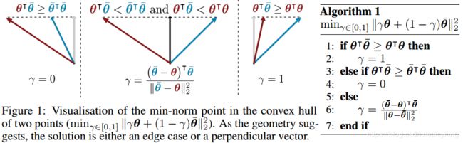
问题(3)等同于在输入点构成的凸包上找一个最小范数的点。这个问题被广泛的研究过，他们假设输入点很多，点的维度很低。但在MTL的问题中，输入点是任务数，往往很少，点的维度是共享的参数数，数量很大。作者提出了新的优化方法，利用Frank-Wolfe algorithm。
总的算法如下图algorithm2所示。

针对Encoder-Decoder Architectures的进一步优化

注意到算法2需要对每个任务的计算${\Delta }_{{\theta }^{sh}}\hat{\mathcal{L}}({\theta }^{sh},{\theta }^t)$，也就需要对共享参数做T次反向传播。这导致一个前向传播后需要T次反向传播。作者提出算法优化上界，使得一次前向传播只需要一次后向传播。
这需要对模型的结构做一定的假设。假设模型有下面的结构：

也就是先经过共享参数的函数$g$，再通过各支任务相关的函数$f^t$。定义$Z=(z_1,\dots ,z_N)$，其中$z_i=g(x_i;{\theta }^{sh})$。使用链式法则可以得到

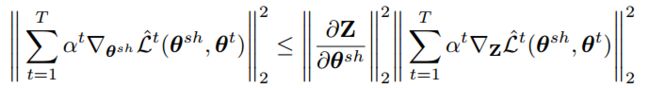
使用上界替换，并去掉常数项，问题(3)变为MGDA-UB (Multiple Gradient Descent Algorithm – Upper Bound)

虽然MGDA-UB是原问题的近似，但作者证明，在温和的假设下，可以得到帕累托最优解：

一些论文中遇到的名词

inductive bias

https://en.wikipedia.org/wiki/Inductive_bias
对于训练样本，就是做拟合，但是未见样本怎么去预测呢？需要一定的假设条件。
对未见样本做预测时使用的假设条件。比如SVM中，最大化margin；KNN中，假设特征空间中近邻的样本有相同的类别。

Pareto optimal

https://en.wikipedia.org/wiki/Pareto_efficiency
帕累托最优所指的情况要求有多个优化目标，指的是不能在不损失其他目标的情况下优化一个目标。

Frank-Wolfe algorithm

https://en.wikipedia.org/wiki/Frank–Wolfe_algorithm
一阶迭代优化算法，优化带约束的凸函数。
收敛速度sublinear。

While competing methods such as gradient descent for constrained optimization require a projection step back to the feasible set in each iteration, the Frank–Wolfe algorithm only needs the solution of a linear problem over the same set in each iteration, and automatically stays in the feasible set.