恐怖袭击等级预测量化与ARMIA时间序列建模的例子

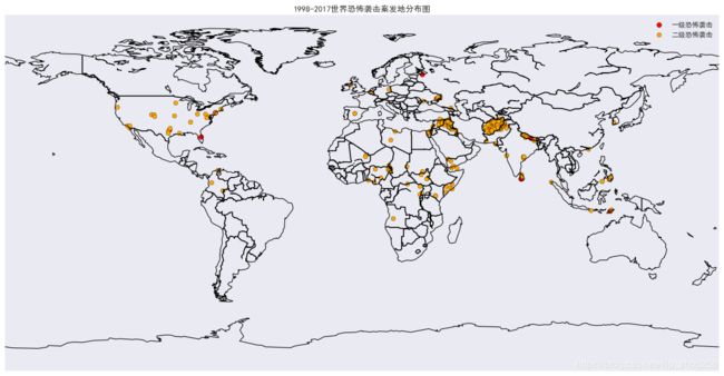
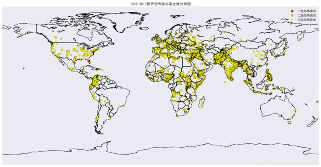
一.恐怖袭击的全球分布量化图:(量化分类由k-means算法得)

# coding:utf-8

import pandas as pd
import mpl_toolkits.basemap             #地图只在Spyder中加载是成功的!!!
import matplotlib.pyplot as plt
import seaborn as sns

plt.style.use('classic')  # 此句设置出雨林绿和中天蓝
#sns.set()

data_file1 = "../data/附件1.xlsx"
data_file2 = "../temp/q1_聚类分级结果.xlsx"
df1 = pd.read_excel(data_file1)    #内含经纬度数据
df2 = pd.read_excel(data_file2)    #量化分级的数据F值和分级
dfdf = pd.merge(df1, df2)
columns1 = dfdf.columns.tolist()
dfdf = dfdf[["eventid", "latitude", "longitude", "F值", "分级"]]

plt.subplots(figsize=(20, 9))
basemap = mpl_toolkits.basemap.Basemap()
basemap.drawcoastlines()
basemap.drawcountries(linewidth=1.5)

# cm = plt.cm.get_cmap('gist_rainbow')
# 直接将聚类的簇号(按照簇的大小来量化分级,簇越大袭击的等级越低)赋给颜色作为能量渐变值
colors = {1: 'red', 2: 'orange', 3: 'yellow', 4: 'cyan', 5: 'green'}
dengji = {1: '一级恐怖袭击', 2: '二级恐怖袭击', 3: '三级恐怖袭击', 4: '四级恐怖袭击', 5: '五级恐怖袭击'}
daxiao = {1: 50, 2: 40, 3: 30, 4: 10, 5: 3}
for i in range(len(colors)):
    px = dfdf['longitude'][dfdf["分级"] == i + 1]
    py = dfdf['latitude'][dfdf["分级"] == i + 1]
    plt.scatter(px, py, c=colors[i + 1], vmin=0, vmax=20000, s=daxiao[i + 1], label=dengji[i + 1])
    # plt.scatter(dfdf['longitude'], dfdf['latitude'], c=dfdf["分级"].apply(lambda x:colors[x]), vmin=0, vmax=200, s=9)
    plt.rcParams['font.sans-serif'] = ['SimHei']  # 标题不能显示汉字,这么处理
    plt.title('1998-2017世界恐怖袭击案发地分布图')
    plt.legend()  # 这里怎么写???
    plt.savefig('../img/world'+str(i)+'.png')
    #plt.show()

效果图:

二.ARMIA时间序列例程

例1：CO2回归预测

"""例1:时间序列建模:ARIMA(差分自回归移动平均模型)"""          
import warnings
import itertools
import pandas as pd
import numpy as np
import statsmodels.api as sm
import matplotlib.pyplot as plt
plt.style.use('fivethirtyeight')
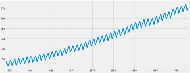
data = sm.datasets.co2.load_pandas()
y = data.data 
y.plot(figsize=(15, 6))
plt.show()      

#1.数据预处理。 每周数据可能很棘手，因为它是一个很短的时间，所以让我们使用每月平均值。 我们将使用resample函数进行转换。 为了简单起见，我们还可以使用fillna()函数来确保我们的时间序列中没有缺少值 
# The 'MS' string groups the data in buckets by start of the month
y = y['co2'].resample('MS').mean()    #将数据按月分组取平均(这是一种累加或者累减的思想)
# The term bfill means that we use the value before filling in missing values
y = y.fillna(y.bfill()) #使用缺失值的前一个来做填充
print(y)  
# 注：y.shape从(2284,1) -> (526,)

#2.探索这个时间序列e作为数据可视化：
y.plot(figsize=(15, 6))
plt.show()

#3.ARIMA时间序列模型调参
# Define the p, d and q parameters to take any value between 0 and 2
p = d = q = range(0, 2)
 
# Generate all different combinations of p, q and q triplets
pdq = list(itertools.product(p, d, q))
"""
	[(0, 0, 0),
	 (0, 0, 1),
	 (0, 1, 0),
	 (0, 1, 1),
	 (1, 0, 0),
	 (1, 0, 1),
	 (1, 1, 0),
	 (1, 1, 1)]
""" 
#3.ARIMA时间序列模型调参
# Define the p, d and q parameters to take any value between 0 and 2
p = d = q = range(0, 2)
 
# Generate all different combinations of p, q and q triplets
pdq = list(itertools.product(p, d, q))
 
# Generate all different combinations of seasonal p, q and q triplets
#产生000--111的8个二进制编码
seasonal_pdq = [(x[0], x[1], x[2], 12) for x in list(itertools.product(p, d, q))]
 
print('Examples of parameter combinations for Seasonal ARIMA...')
print('SARIMAX: {} x {}'.format(pdq[1], seasonal_pdq[1]))
print('SARIMAX: {} x {}'.format(pdq[1], seasonal_pdq[2]))
print('SARIMAX: {} x {}'.format(pdq[2], seasonal_pdq[3]))
print('SARIMAX: {} x {}'.format(pdq[2], seasonal_pdq[4]))

# 使用网格搜索，我们已经确定了为我们的时间序列数据生成最佳拟合模型的参数集。 我们可以更深入地分析这个特定的模型。 
warnings.filterwarnings("ignore") # specify to ignore warning messages
for param in pdq:
    for param_seasonal in seasonal_pdq:
        try:
            mod = sm.tsa.statespace.SARIMAX(y,
                                            order=param,
                                            seasonal_order=param_seasonal,
                                            enforce_stationarity=False,
                                            enforce_invertibility=False)
 
            results = mod.fit()
 
            print('ARIMA{}x{}12 - AIC:{}'.format(param, param_seasonal, results.aic))
        except:
            continue
# 我们的代码的输出表明， SARIMAX(1, 1, 1)x(1, 1, 1, 12)产生最低的AIC值为277.78。 因此，我们认为这是我们考虑过的所有模型中的最佳选择。 

#我们首先将最佳参数值插入到新的SARIMAX模型中
mod = sm.tsa.statespace.SARIMAX(y,
                                order=(1, 1, 1),
                                seasonal_order=(1, 1, 1, 12),
                                enforce_stationarity=False,
                                enforce_invertibility=False)
 
results = mod.fit()
print(results.summary().tables[1])
# coef列显示每个特征的重量（即重要性）以及每个特征如何影响时间序列
# P>|z| 列通知我们每个特征重量的意义。 这里，每个重量的p值都低于或接近0.05 ，所以在我们的模型中保留所有权重是合理的

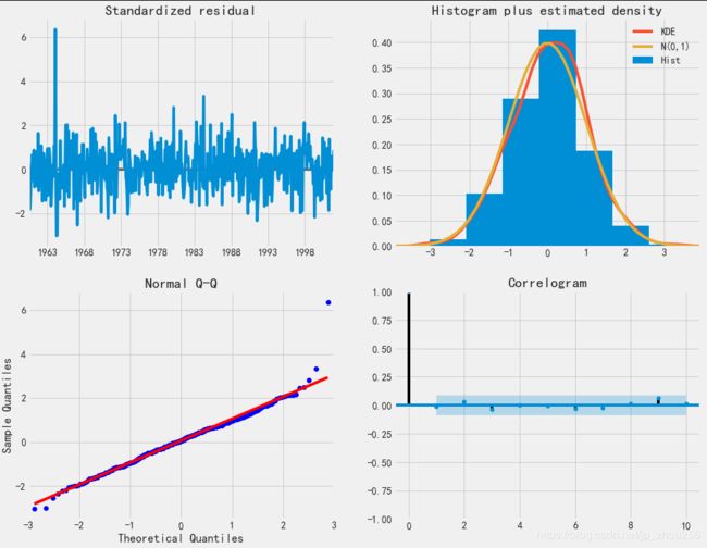
#在适合季节性ARIMA模型（以及任何其他模型）的情况下，运行模型诊断是非常重要的，以确保没有违反模型的假设。 plot_diagnostics对象允许我们快速生成模型诊断并调查任何异常行为
results.plot_diagnostics(figsize=(15, 12))
plt.show()

# 我们的主要关切是确保我们的模型的残差是不相关的，并且平均分布为零。 如果季节性ARIMA模型不能满足这些特性，这是一个很好的迹象，可以进一步改善。 
#在这种情况下，我们的模型诊断表明，模型残差正常分布如下：
#在右上图中，我们看到红色KDE线与N(0,1)行（其中N(0,1) ）是正态分布的标准符号，平均值0 ，标准偏差为1 ） 。 这是残留物正常分布的良好指示。
#左下角的qq图显示，残差（蓝点）的有序分布遵循采用N(0, 1)的标准正态分布采样的线性趋势。 同样，这是残留物正常分布的强烈指示。
#随着时间的推移（左上图）的残差不会显示任何明显的季节性，似乎是白噪声。 这通过右下角的自相关（即相关图）来证实，这表明时间序列残差与其本身的滞后版本具有低相关性。 
#这些观察结果使我们得出结论，我们的模型产生了令人满意的合适性，可以帮助我们了解我们的时间序列数据和预测未来价值。
#虽然我们有一个令人满意的结果，我们的季节性ARIMA模型的一些参数可以改变，以改善我们的模型拟合。 例如，我们的网格搜索只考虑了一组受限制的参数组合，所以如果我们拓宽网格搜索，我们可能会找到更好的模型。 

#我们已经获得了我们时间序列的模型，现在可以用来产生预测
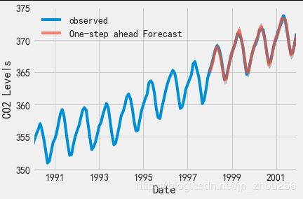
#我们首先将预测值与时间序列的实际值进行比较，这将有助于我们了解我们的预测的准确性。 get_prediction()和conf_int()属性允许我们获得时间序列预测的值和相关的置信区间。
pred = results.get_prediction(start=pd.to_datetime('1998-01-01'), dynamic=False)
pred_ci = pred.conf_int()
# 上述规定需要从1998年1月开始进行预测。
#dynamic=False参数确保我们产生一步前进的预测，这意味着每个点的预测都将使用到此为止的完整历史生成。
#我们可以绘制二氧化碳时间序列的实际值和预测值，以评估我们做得如何。 注意我们如何在时间序列的末尾放大日期索引。 
ax = y['1990':].plot(label='observed')
pred.predicted_mean.plot(ax=ax, label='One-step ahead Forecast', alpha=.7)
 
ax.fill_between(pred_ci.index,
                pred_ci.iloc[:, 0],
                pred_ci.iloc[:, 1], color='k', alpha=.2)
 
ax.set_xlabel('Date')
ax.set_ylabel('CO2 Levels')
plt.legend()
plt.show()
#总体而言，我们的预测与真实价值保持一致，呈现总体增长趋势。

# 量化我们的预测的准确性也是有用的,使用MSE（均方误差）.
y_forecasted = pred.predicted_mean
y_truth = y['1998-01-01':]
 
# Compute the mean square error
mse = ((y_forecasted - y_truth) ** 2).mean()
print('The Mean Squared Error of our forecasts is {}'.format(round(mse, 2)))

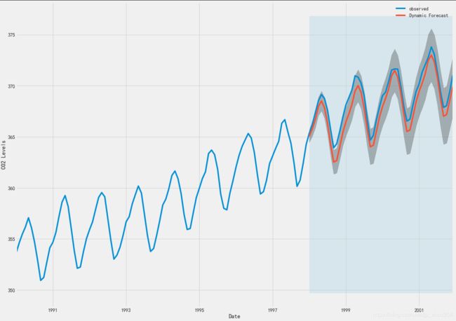
# 然而，使用【动态预测】可以获得更好地表达我们的真实预测能力。 在这种情况下，我们只使用时间序列中的信息到某一点，之后，使用先前预测时间点的值生成预测。 
pred_dynamic = results.get_prediction(start=pd.to_datetime('1998-01-01'), dynamic=True, full_results=True)
pred_dynamic_ci = pred_dynamic.conf_int()

#绘制时间序列的观测值和预测值，我们看到即使使用动态预测，总体预测也是准确的。 所有预测值（红线）与地面真相（蓝线）相当吻合，并且在我们预测的置信区间内
ax = y['1990':].plot(label='observed', figsize=(20, 15))
pred_dynamic.predicted_mean.plot(label='Dynamic Forecast', ax=ax)
ax.fill_between(pred_dynamic_ci.index,
                pred_dynamic_ci.iloc[:, 0],
                pred_dynamic_ci.iloc[:, 1], color='k', alpha=.25)
ax.fill_betweenx(ax.get_ylim(), pd.to_datetime('1998-01-01'), y.index[-1],
                 alpha=.1, zorder=-1)
ax.set_xlabel('Date')
ax.set_ylabel('CO2 Levels')
plt.legend()
plt.show()

#再次通过计算MSE量化我们预测的预测性能：
# Extract the predicted and true values of our time-series
y_forecasted = pred_dynamic.predicted_mean
y_truth = y['1998-01-01':]
# Compute the mean square error
mse = ((y_forecasted - y_truth) ** 2).mean()
print('The Mean Squared Error of our forecasts is {}'.format(round(mse, 2)))

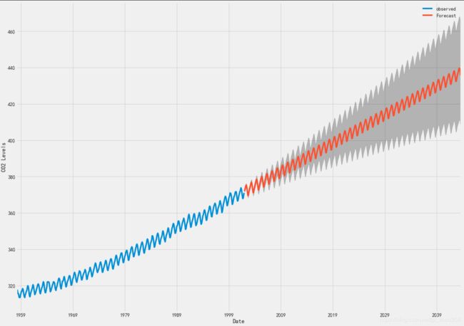
#然而，关于时间序列预测的大部分兴趣是能够及时预测未来价值观。
#利用季节性ARIMA时间序列模型来预测未来的价值。 我们的时间序列对象的get_forecast()属性可以计算预先指定数量的步骤的预测值。
# Get forecast 500 steps ahead in future
pred_uc = results.get_forecast(steps=500)
# Get confidence intervals of forecasts
pred_ci = pred_uc.conf_int()
#输出绘制其未来值的时间序列和预测。
ax = y.plot(label='observed', figsize=(20, 15))
pred_uc.predicted_mean.plot(ax=ax, label='Forecast')
ax.fill_between(pred_ci.index,
                pred_ci.iloc[:, 0],
                pred_ci.iloc[:, 1], color='k', alpha=.25)
ax.set_xlabel('Date')
ax.set_ylabel('CO2 Levels')
plt.legend()
plt.show()
# 现在可以使用我们生成的预测和相关的置信区间来进一步了解时间序列并预见预期。 我们的预测显示，时间序列预计将继续稳步增长。 

Examples of parameter combinations for Seasonal ARIMA...
SARIMAX: (0, 0, 1) x (0, 0, 1, 12)
SARIMAX: (0, 0, 1) x (0, 1, 0, 12)
SARIMAX: (0, 1, 0) x (0, 1, 1, 12)
SARIMAX: (0, 1, 0) x (1, 0, 0, 12)
ARIMA(0, 0, 0)x(0, 0, 1, 12)12 - AIC:6787.343624043257
ARIMA(0, 0, 0)x(0, 1, 1, 12)12 - AIC:1596.7111727638858
ARIMA(0, 0, 0)x(1, 0, 0, 12)12 - AIC:1058.9388921320021
ARIMA(0, 0, 0)x(1, 0, 1, 12)12 - AIC:1056.2878545588537
ARIMA(0, 0, 0)x(1, 1, 0, 12)12 - AIC:1361.65789780726
ARIMA(0, 0, 0)x(1, 1, 1, 12)12 - AIC:1044.7647912955827
ARIMA(0, 0, 1)x(0, 0, 0, 12)12 - AIC:6881.048754598261
ARIMA(0, 0, 1)x(0, 0, 1, 12)12 - AIC:6072.662327394357
ARIMA(0, 0, 1)x(0, 1, 0, 12)12 - AIC:1379.1941067304665
ARIMA(0, 0, 1)x(0, 1, 1, 12)12 - AIC:1241.4174716865425
ARIMA(0, 0, 1)x(1, 0, 0, 12)12 - AIC:1105.710323856536
ARIMA(0, 0, 1)x(1, 0, 1, 12)12 - AIC:780.4315876419755
ARIMA(0, 0, 1)x(1, 1, 0, 12)12 - AIC:1119.5957893641971
ARIMA(0, 0, 1)x(1, 1, 1, 12)12 - AIC:807.091298905328
ARIMA(0, 1, 0)x(0, 0, 1, 12)12 - AIC:1240.2211199194103
ARIMA(0, 1, 0)x(0, 1, 1, 12)12 - AIC:337.79385497181556
ARIMA(0, 1, 0)x(1, 0, 0, 12)12 - AIC:619.950175782907
ARIMA(0, 1, 0)x(1, 0, 1, 12)12 - AIC:376.928375962471
ARIMA(0, 1, 0)x(1, 1, 0, 12)12 - AIC:478.32969081693074
ARIMA(0, 1, 0)x(1, 1, 1, 12)12 - AIC:323.3246684714404
ARIMA(0, 1, 1)x(0, 0, 0, 12)12 - AIC:1371.187260233532
ARIMA(0, 1, 1)x(0, 0, 1, 12)12 - AIC:1101.8410734303063
ARIMA(0, 1, 1)x(0, 1, 0, 12)12 - AIC:587.9479710198574
ARIMA(0, 1, 1)x(0, 1, 1, 12)12 - AIC:302.4949004407664
ARIMA(0, 1, 1)x(1, 0, 0, 12)12 - AIC:584.4333533197422
ARIMA(0, 1, 1)x(1, 0, 1, 12)12 - AIC:337.1999050859573
ARIMA(0, 1, 1)x(1, 1, 0, 12)12 - AIC:433.0863608138467
ARIMA(0, 1, 1)x(1, 1, 1, 12)12 - AIC:281.51901861696274
ARIMA(1, 0, 0)x(0, 0, 0, 12)12 - AIC:1676.8881767362052
ARIMA(1, 0, 0)x(0, 0, 1, 12)12 - AIC:1241.9354688169774
ARIMA(1, 0, 0)x(0, 1, 0, 12)12 - AIC:624.2602350563734
ARIMA(1, 0, 0)x(0, 1, 1, 12)12 - AIC:341.28966096085986
ARIMA(1, 0, 0)x(1, 0, 0, 12)12 - AIC:579.3896095902396
ARIMA(1, 0, 0)x(1, 0, 1, 12)12 - AIC:370.5917481686993
ARIMA(1, 0, 0)x(1, 1, 0, 12)12 - AIC:476.0500429294359
ARIMA(1, 0, 0)x(1, 1, 1, 12)12 - AIC:329.5844991609267
ARIMA(1, 0, 1)x(0, 0, 0, 12)12 - AIC:1372.6085881642894
ARIMA(1, 0, 1)x(0, 0, 1, 12)12 - AIC:1199.4888120556775
ARIMA(1, 0, 1)x(0, 1, 0, 12)12 - AIC:586.4485732463568
ARIMA(1, 0, 1)x(0, 1, 1, 12)12 - AIC:305.6273820506816
ARIMA(1, 0, 1)x(1, 0, 0, 12)12 - AIC:586.5104873326288
ARIMA(1, 0, 1)x(1, 0, 1, 12)12 - AIC:390.01257894365034
ARIMA(1, 0, 1)x(1, 1, 0, 12)12 - AIC:433.5469464372751
ARIMA(1, 0, 1)x(1, 1, 1, 12)12 - AIC:284.3596617065916
ARIMA(1, 1, 0)x(0, 0, 0, 12)12 - AIC:1324.311112732457
ARIMA(1, 1, 0)x(0, 0, 1, 12)12 - AIC:1060.9351914429194
ARIMA(1, 1, 0)x(0, 1, 0, 12)12 - AIC:600.7412682874252
ARIMA(1, 1, 0)x(0, 1, 1, 12)12 - AIC:312.13296334793273
ARIMA(1, 1, 0)x(1, 0, 0, 12)12 - AIC:593.6637754555269
ARIMA(1, 1, 0)x(1, 0, 1, 12)12 - AIC:349.20913954048615
ARIMA(1, 1, 0)x(1, 1, 0, 12)12 - AIC:440.13758839992397
ARIMA(1, 1, 0)x(1, 1, 1, 12)12 - AIC:293.742622285657
ARIMA(1, 1, 1)x(0, 0, 0, 12)12 - AIC:1262.6545542464787
ARIMA(1, 1, 1)x(0, 0, 1, 12)12 - AIC:1052.0636724059154
ARIMA(1, 1, 1)x(0, 1, 0, 12)12 - AIC:581.3099935196991
ARIMA(1, 1, 1)x(0, 1, 1, 12)12 - AIC:295.9374060570654
ARIMA(1, 1, 1)x(1, 0, 0, 12)12 - AIC:576.864711171842
ARIMA(1, 1, 1)x(1, 0, 1, 12)12 - AIC:327.90491258388
ARIMA(1, 1, 1)x(1, 1, 0, 12)12 - AIC:444.12436865303255
ARIMA(1, 1, 1)x(1, 1, 1, 12)12 - AIC:277.78021986187264

==============================================================================
                 coef    std err          z      P>|z|      [0.025      0.975]
------------------------------------------------------------------------------
ar.L1          0.3182      0.092      3.442      0.001       0.137       0.499
ma.L1         -0.6254      0.077     -8.162      0.000      -0.776      -0.475
ar.S.L12       0.0010      0.001      1.732      0.083      -0.000       0.002
ma.S.L12      -0.8769      0.026    -33.812      0.000      -0.928      -0.826
sigma2         0.0972      0.004     22.632      0.000       0.089       0.106
==============================================================================

注：长周期数据，Q-Q往往会有很好的线性表现。

例2：茅台股票走势预测

"""例2:时间序列建模:ARIMA(差分自回归移动平均模型)"""  
import tushare as ts
import warnings
import pandas as pd
import numpy as np
import datetime
import statsmodels.api as sm
from dateutil.parser import parse
import matplotlib.pyplot as plt
import seaborn as sns
from statsmodels.tsa.arima_model import ARIMA
from statsmodels.graphics.tsaplots import plot_acf, plot_pacf
warnings.filterwarnings('ignore')
plt.rcParams['font.sans-serif'] = ['SimHei'] # 设置字体为黑体
plt.rcParams['axes.unicode_minus'] = False # 解决中文字体负号显示不正常问题 
sns.set_style("whitegrid",{"font.sans-serif":['KaiTi', 'Arial']})

#获取股票代号为600519的茅台股票数据
k  = ts.get_hist_data('600519') #600519茅台股票  这里可以设置获取的时间段
# k  = ts.get_hist_data('600519',start='2015-05-04',end='2018-05-02') #指定具体的起始时间
 
lit = ['open', 'high', 'close', 'low']  #这里我们只获取其中四列
data = k[lit]
 
d_one = data.index      #以下9行将object的index转换为datetime类型
d_two = []
d_three = []
date2 = []
for i in d_one:
    d_two.append(i)
for i in range(len(d_two)):
    d_three.append(parse(d_two[i]))
data2 = pd.DataFrame(data,index=d_three,dtype=np.float64)   #构建新的DataFrame赋予index为转换的d_three。当然你也可以使用date_range()来生成时间index
 
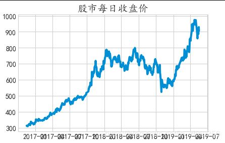
plt.plot(data2['close'])    #一看数据就不稳定，所以我们需要做差分
plt.title('股市每日收盘价')
plt.show()
 
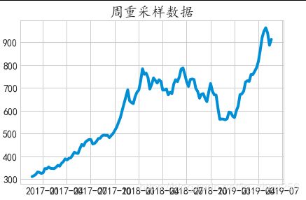
data2_w = data2['close'].resample('W-MON').mean()   #由于原始数据太多，按照每一周来采样，更好预测，并取每一周的均值
#data2_train是我要预测的内容
#data2_train = data2_w['2015':'2017']    #我们只取2015到2017的数据来训练
data2_train = data2_w['2015':'2019']    #我们只取2015到2019的数据来训练,长周期表现出来了更好的回归预测性能.
plt.plot(data2_train)
plt.title('周重采样数据')
plt.show()
 
#一阶差分，分析ACF
acf = plot_acf(data2_train,lags=20)     #通过plot_acf来查看训练数据，以便我们判断q的取值
plt.title("股票指数的 ACF")
acf.show()
 
#一阶差分，分析PACF
pacf = plot_pacf(data2_train,lags=20)   #通过plot_pacf来查看训练数据，以便我们判断p的取值
plt.title("股票指数的 PACF")
pacf.show()
 
#处理数据，平稳化处理
data2_diff = data2_train.diff(1)    #差分很简单使用pandas的diff()函数可以进行一阶差分
diff = data2_diff.dropna()
for i in range(2):          #五阶差分，一般一到二阶就行了，我有点过分
    diff = diff.diff(1)
    diff = diff.dropna()
plt.figure()
plt.plot(diff)
plt.title('五阶差分')
plt.show()
 
# 五阶差分的ACF
acf_diff = plot_acf(diff,lags=20)
plt.title("五阶差分的ACF")         #根据ACF图，观察来判断q
acf_diff.show()
 
# 五阶差分的PACF
pacf_diff = plot_pacf(diff,lags=20)   #根据PACF图，观察来判断p
plt.title("五阶差分的PACF")
pacf_diff.show()
 
mod = sm.tsa.statespace.SARIMAX(data2_train,
                            order=(1, 1, 1),
                            seasonal_order=(1, 1, 1, 12),
                            enforce_stationarity=False,
                            enforce_invertibility=False)
results = mod.fit()
print(results.summary().tables[1])
# coef列显示每个特征的重量（即重要性）以及每个特征如何影响时间序列
# P>|z| 列通知我们每个特征重量的意义。 这里，每个重量的p值都低于或接近0.05 ，所以在我们的模型中保留所有权重是合理的

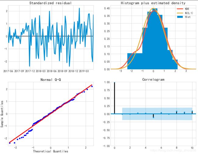
#在适合季节性ARIMA模型（以及任何其他模型）的情况下，运行模型诊断是非常重要的，以确保没有违反模型的假设。 plot_diagnostics对象允许我们快速生成模型诊断并调查任何异常行为
results.plot_diagnostics(figsize=(15, 12))
plt.show()
#我们首先将预测值与时间序列的实际值进行比较，这将有助于我们了解我们的预测的准确性。 get_prediction()和conf_int()属性允许我们获得时间序列预测的值和相关的置信区间。
pred = results.get_prediction(start=pd.to_datetime('2016-12-05'), dynamic=False)
pred_ci = pred.conf_int()

pred_uc = results.get_forecast(steps=500)
# Get confidence intervals of forecasts
pred_ci = pred_uc.conf_int()
# 上述规定需要从1998年1月开始进行预测。
#dynamic=False参数确保我们产生一步前进的预测，这意味着每个点的预测都将使用到此为止的完整历史生成。
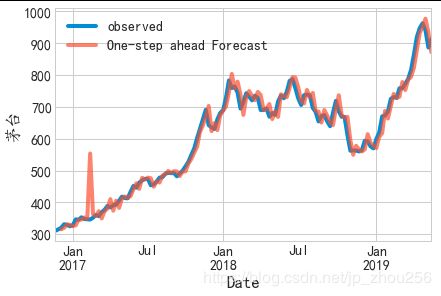
#绘制茅台时间序列的实际值和预测值，以评估我们做得如何。 注意我们如何在时间序列的末尾放大日期索引。 
ax = data2_train['2016':].plot(label='observed')
pred.predicted_mean.plot(ax=ax, label='One-step ahead Forecast', alpha=.7)
ax.set_xlabel('Date')
ax.set_ylabel('茅台')
plt.legend()
plt.show() 


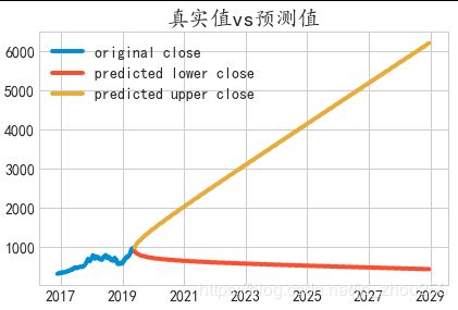
#可视化预测
stock_forcast = pd.concat([data2_w,pred_ci],axis=1,keys=['original', 'predicted'])   #将原始数据和预测数据相结合，使用keys来分层
 
#构图
plt.figure()
stock_forcast.columns.tolist()
stock_forcast.columns=["original","lowerclose","upperclose"]
s1=stock_forcast["original"]
s2=stock_forcast["lowerclose"]
s3=stock_forcast["upperclose"]
plt.plot(s1,label="original close")
plt.plot(s2,label="predicted lower close")
plt.plot(s3,label="predicted upper close")
plt.title('真实值vs预测值')
plt.legend()
plt.show()

==============================================================================
                 coef    std err          z      P>|z|      [0.025      0.975]
------------------------------------------------------------------------------
ar.L1         -0.0993      0.248     -0.401      0.688      -0.585       0.386
ma.L1          0.4512      0.244      1.850      0.064      -0.027       0.929
ar.S.L12      -0.0030      0.088     -0.034      0.973      -0.176       0.170
ma.S.L12      -1.0000   2513.778     -0.000      1.000   -4927.915    4925.915
sigma2       514.1104   1.29e+06      0.000      1.000   -2.53e+06    2.53e+06
==============================================================================

#data2_train = data2_w[‘2015’:‘2017’] #我们只取2015到2017的数据来训练

data2_train = data2_w[‘2015’:‘2019’] #我们只取2015到2019的数据来训练,长周期表现出来了更好

例3：使用LSTM模型来预测国际机场人流量
数据集(international-airline-passengers.csv)下载地址：
英文例子：
https://machinelearningmastery.com/time-series-prediction-lstm-recurrent-neural-networks-python-keras/

中文例子：
https://www.jianshu.com/p/38df71cad1f6

"""例3:LSTM模型预测时间序列数据:机场乘客流量预测"""
import numpy
import matplotlib.pyplot as plt
from pandas import read_csv
import math
from keras.models import Sequential
from keras.layers import Dense
from keras.layers import LSTM
from sklearn.preprocessing import MinMaxScaler
from sklearn.metrics import mean_squared_error
#访问英文网址链接,替换掉所有"",然后Excel中"数据">"来自文本数据">","分隔
dataframe = read_csv('C:/Users/Administrator/Desktop/4508AF00.csv', usecols=[1], engine='python', skipfooter=3)
dataset = dataframe.values
# 将整型变为float
dataset = dataset.astype('float32')
 
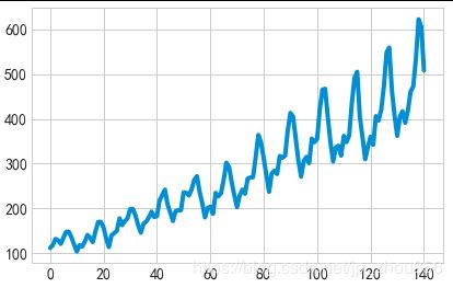
plt.plot(dataset)
plt.show()

#将一列变成两列，第一列是第 t 月的乘客数，第二列是第 t+1 月的乘客数。 look_back 就是预测下一步所需要的 timesteps
#timesteps 就是 LSTM 认为每个输入数据与前多少个陆续输入的数据有联系。例如具有这样用段序列数据 “…ABCDBCEDF…”，当 timesteps 为 3 时，在模型预测中如果输入数据为“D”，那么之前接收的数据如果为“B”和“C”则此时的预测输出为 B 的概率更大，之前接收的数据如果为“C”和“E”，则此时的预测输出为 F 的概率更大。
# X is the number of passengers at a given time (t) 
#and Y is the number of passengers at the next time (t + 1).
 
# convert an array of values into a dataset matrix
def create_dataset(dataset, look_back=1):
    dataX, dataY = [], []
    for i in range(len(dataset)-look_back-1):
        a = dataset[i:(i+look_back), 0]
        dataX.append(a)
        dataY.append(dataset[i + look_back, 0])
    return numpy.array(dataX), numpy.array(dataY)
 
# fix random seed for reproducibility
numpy.random.seed(7)

#当激活函数为 sigmoid 或者 tanh 时，要把数据正则话，此时 LSTM 比较敏感 设定 67% 是训练数据，余下的是测试数据
# normalize the dataset
scaler = MinMaxScaler(feature_range=(0, 1))
dataset = scaler.fit_transform(dataset)
 
 
# split into train and test sets
train_size = int(len(dataset) * 0.67)
test_size = len(dataset) - train_size
train, test = dataset[0:train_size,:], dataset[train_size:len(dataset),:]
#X=t and Y=t+1 时的数据，并且此时的维度为 [samples, features]
# use this function to prepare the train and test datasets for modeling
look_back = 1
trainX, trainY = create_dataset(train, look_back)
testX, testY = create_dataset(test, look_back)
#投入到 LSTM 的 X 需要有这样的结构： [samples, time steps, features]，所以做一下变换
# reshape input to be [samples, time steps, features]
trainX = numpy.reshape(trainX, (trainX.shape[0], 1, trainX.shape[1]))
testX = numpy.reshape(testX, (testX.shape[0], 1, testX.shape[1]))
#建立 LSTM 模型： 输入层有 1 个input，隐藏层有 4 个神经元，输出层就是预测一个值，激活函数用 sigmoid，迭代 100 次，batch size 为 1
#create and fit the LSTM network
model = Sequential()
#model.add(LSTM(24, input_shape=(1, look_back)))
model.add(LSTM(units=256,input_shape=(None,1),return_sequences=True))
model.add(LSTM(units=256))
model.add(Dense(1))
model.compile(loss='mean_squared_error', optimizer='adam')
model.fit(trainX, trainY, epochs=100, batch_size=1, verbose=2)
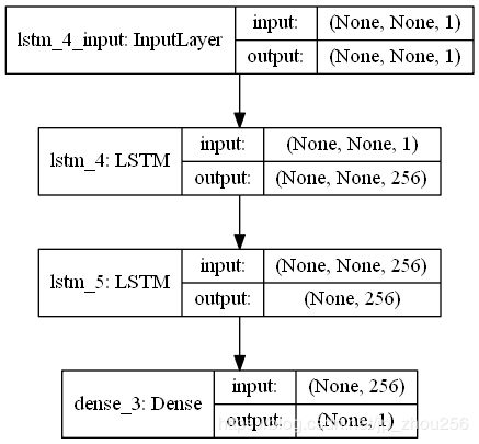
# 绘制网络结构
plot_model(model, to_file='E:/model.png', show_shapes=True);

#预测：
# make predictions
trainPredict = model.predict(trainX)
testPredict = model.predict(testX)
#计算误差之前要先把预测数据转换成同一单位
# invert predictions
trainPredict = scaler.inverse_transform(trainPredict)
trainY = scaler.inverse_transform([trainY])
testPredict = scaler.inverse_transform(testPredict)
testY = scaler.inverse_transform([testY])

#计算 mean squared error
trainScore = math.sqrt(mean_squared_error(trainY[0], trainPredict[:,0]))
print('Train Score: %.2f RMSE' % (trainScore))
testScore = math.sqrt(mean_squared_error(testY[0], testPredict[:,0]))
print('Test Score: %.2f RMSE' % (testScore))

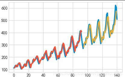
#画出结果：蓝色为原数据，绿色为训练集的预测值，红色为测试集的预测值
# shift train predictions for plotting
trainPredictPlot = numpy.empty_like(dataset)
trainPredictPlot[:, :] = numpy.nan
trainPredictPlot[look_back:len(trainPredict)+look_back, :] = trainPredict
 
# shift test predictions for plotting
testPredictPlot = numpy.empty_like(dataset)
testPredictPlot[:, :] = numpy.nan
testPredictPlot[len(trainPredict)+(look_back*2)+1:len(dataset)-1, :] = testPredict
 
# plot baseline and predictions
plt.plot(scaler.inverse_transform(dataset))
plt.plot(trainPredictPlot)
plt.plot(testPredictPlot)
plt.show()

注:# 绘制网络结构(安装pydot教程)
plot_model(model, to_file=‘E:/model.png’, show_shapes=True);

首先下载 pydotplus 包。
>pip install pydotplus

然后找到 pydotplus 包的存储位置，将包名更改为pydot (会有两个文件包，pydotplus 和 pydotplus-2.0.2.dist-info , 只要修改前一个包名就可以了)。例如我的存储位置在D:\Anaconda3\Lib\site-packages\pydotplus , 修改为D:\Anaconda3\Lib\site-packages\pydot。

再打开 pydot 文件夹中的 parser.py文件，将
import pydotplus 
修改为
import pydot

运行程序，再次报错。
pydot.InvocationException: GraphViz's executables not found

打开 pydot 文件夹中的 graphviz.py文件，找到 find_graphviz() 函数。将
#Method 3 (Windows only)

这行之后的代码替换为下列代码。
    # Method 3 (Windows only)
    #
    if os.sys.platform == 'win32':
        # Try and work out the equivalent of "C:\Program Files" on this
        # machine (might be on drive D:, or in a different language)
        #
        if False:  # os.environ.has_key('PROGRAMFILES'):      #######################修改这里
            # Note, we could also use the win32api to get this
            # information, but win32api may not be installed.
            path = os.path.join(os.environ['PROGRAMFILES'], 'ATT', 'GraphViz', 'bin')
        else:
            # Just in case, try the default...
            path = r"D:\Graphviz\bin"          ########################修改这里
        progs = __find_executables(path)
     
        if progs is not None:
            # print "Used default install location"
            return progs
     
    for path in (
            '/usr/bin', '/usr/local/bin',
            '/opt/bin', '/sw/bin', '/usr/share',
            '/Applications/Graphviz.app/Contents/MacOS/'):
        progs = __find_executables(path)
     
        if progs is not None:
            # print "Used path"
            return progs
    # Failed to find GraphViz
    #
    return None

其中 D:\Graphviz\bin 是 Graphviz 软件在我电脑上的安装路径，将其更改为你的安装路径。
到这里应该安装成功了，运行程序就能输出模型图了。

例4：LSTM用于空气质量的多变量回归预测()
空气质量数据集。数据来源自位于北京的美国大使馆在2010年至2014年共5年间每小时采集的天气及空气污染指数。 数据集中的多变量(属性、特征)如下所示：

1.No 行数
2.year 年
3.month 月
4.day 日
5.hour 小时
6.pm2.5 PM2.5浓度
7.DEWP 露点
8.TEMP 温度
9.PRES 大气压
10.cbwd 风向
11.lws 风速
12.ls 累积雪量
13.lr 累积雨量

"""例4:基于LSTM的空气质量的回归预测(多变量、时间序列问题)"""
#1.粗略的观察数据集会发现最开始的24小时PM2.5值都是NA，因此需要删除这部分数据，对于其他时刻少量的缺省值利用Pandas中的fillna填充；同时需要整合日期数据，使其作为Pandas中索引（index）。
#下面的代码完成了以上的处理过程，同时去掉了原始数据中“No”列，并将列命名为更清晰的名字
from pandas import read_csv
from datetime import datetime
import pandas as pd
import numpy as np
from keras.models import Sequential
from keras.layers import Dense
from keras.layers import LSTM
from sklearn.preprocessing import MinMaxScaler
from sklearn.metrics import mean_squared_error
from keras.utils.vis_utils import plot_model

#第一种拼接日期并解析的方式,用于read_csv:year,month,day,hour均被替换不会被保留
def jiexi1(x):
    temp=x.split()
    str1=""
    for i in range(len(temp)-1):
        str1+=temp[i]+"-"
    str1+=" "+temp[len(temp)-1]+':'+str(0)+':'+str(0)
    return str1
    
dateparse = lambda x: jiexi1(x)
#df = pd.read_csv("C:/Users/Administrator/Desktop/lstm-pollution.csv", parse_dates={'datetime':[1,2,3,4]},infer_datetime_format=True)
df = pd.read_csv("C:/Users/Administrator/Desktop/lstm-pollution.csv", parse_dates={'datetime':[1,2,3,4]},date_parser=dateparse)

#第二种拼接日期并解析的方式,用于read_csv():year,month,day,hour均还会保留
#df = pd.read_csv("C:/Users/Administrator/Desktop/lstm-pollution.csv")
#df['year']=df['year'].astype(str)
#df['month']=df['month'].astype(str)
#df['day']=df['day'].astype(str)
#df['hour']=df['hour'].astype(str)
##首先将数值型的year,month,day,hour转为str类型,然后拼接出来日期函数可以识别的模式字符串,使用下列两种方式来做转换操作。
#df['datetime']=(df.year+'-'+df.month+'-'+df.day+' '+df.hour+':'+str(0)+':'+str(0)).apply(lambda x:datetime.strptime(x, '%Y-%m-%d %H:%M:%S')).tolist()
#df['datetime2']=pd.to_datetime(df.year+'-'+df.month+'-'+df.day+' '+df.hour+':'+str(0)+':'+str(0),format='%Y-%m-%d %H:%M:%S')#结果同下


df.drop('No', axis=1, inplace=True)
# manually specify column names
df.columns = ['datetime','pm2.5','DEWP',	'TEMP',	'PRESS','wnd_dir','wnd_spd','snow','rain']

df.index=df['datetime']
del df['datetime']
# mark all NA values with 0
df['pm2.5'].fillna(0, inplace=True)
#删除pm2.5为空的前24行记录
df = df[24:]
df['pm2.5'].values
#删除缺失值所在的行
#df=df.drop(df[df['pm2.5'].values==np.nan].index.tolist())  #删除空值所在的所有行.
#df1=df[~df['pm2.5'].isnull()]
# summarize first 5 rows
print(df.head(5))
# save to file
df.to_csv('C:/Users/Administrator/Desktop/pollution.csv')
 
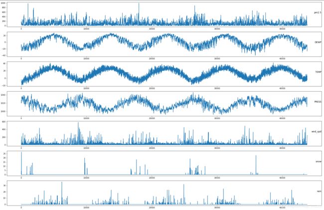
#2.在的数据格式已经更加适合处理，可以简单的对每列进行绘图。下面的代码加载了“pollution.csv”文件，并对除了类别型特性“风速”的每一列数据分别绘图
from pandas import read_csv
from matplotlib import pyplot
from sklearn.preprocessing import LabelEncoder
from sklearn.preprocessing import MinMaxScaler
# load dataset
dataset = read_csv('C:/Users/Administrator/Desktop/pollution.csv', header=0, index_col=0)
values = dataset.values
# specify columns to plot
groups = [0, 1, 2, 3, 5, 6, 7]
i = 1
# plot each column
pyplot.figure(figsize=(30,20))
for group in groups:
    pyplot.subplot(len(groups), 1, i)
    pyplot.plot(values[:, group])
    pyplot.title(dataset.columns[group], y=0.5, loc='right')
    i += 1
pyplot.show()
 
#3.多变量LSTM预测模型
#接着对所有的特征进行归一化处理，然后将数据集转化为有监督学习问题，同时将需要预测的当前时刻（t）的天气条件特征移除
#1. 利用过去24小时的污染数据和天气条件预测当前时刻的污染；
#2. 预测下一个时刻（t+1）可能的天气条件；
# convert series to supervised learning
def series_to_supervised(data, n_in=1, n_out=1, dropnan=True):
    n_vars = 1 if type(data) is list else data.shape[1]
    df = pd.DataFrame(data)
    cols, names = list(), list()
    # input sequence (t-n, ... t-1)
    for i in range(n_in, 0, -1):
        cols.append(df.shift(i))
        names += [('var%d(t-%d)' % (j+1, i)) for j in range(n_vars)]
    # forecast sequence (t, t+1, ... t+n)
    for i in range(0, n_out):
        cols.append(df.shift(-i))
        if i == 0:
            names += [('pm2.5%d(t)' % (j+1)) for j in range(n_vars)]
        else:
            names += [('var%d(t+%d)' % (j+1, i)) for j in range(n_vars)]
    # put it all together
    agg = pd.concat(cols, axis=1)
    agg.columns = names
    # drop rows with NaN values
    if dropnan:
        agg.dropna(inplace=True)
    return agg

# load dataset
dataset = read_csv('C:/Users/Administrator/Desktop/pollution.csv', header=0, index_col=0)
values = dataset.values
dataset.info()
# integer encode direction
encoder = LabelEncoder()  #利用sklearn的预处理模块对类别特征“风向”进行编码，当然也可以对该特征进行one-hot编码。 
values[:,4] = encoder.fit_transform(values[:,4])
# ensure all data is float
values = values.astype('float32')
# normalize features
scaler = MinMaxScaler(feature_range=(0, 1))
scaled = scaler.fit_transform(values)
# frame as supervised learning
reframed = series_to_supervised(scaled, 1, 1)
# drop columns we don't want to predict
reframed.drop(reframed.columns[[9,10,11,12,13,14,15]], axis=1, inplace=True)
print(reframed.head())
#数据集的处理比较简单，还有很多的方式可以尝试，一些可以尝试的方向包括：
#1>对“风向”特征哑编码；
#2>加入季节特征；
#3>时间步长超过1。
#其中，上述第三种方式对于处理时间序列问题的LSTM可能是最重要的。

#3.构造LSTM模型。 
#将处理后的数据集划分为训练集和测试集。为了加速模型的训练，我们仅利用第一年数据进行训练，然后利用剩下的4年进行评估
#将数据集进行划分，然后将训练集和测试集划分为输入和输出变量，最终将输入（X）改造为LSTM的输入格式，即[samples,timesteps,features],如:print(train_X.shape)=(8760, 1, 8)
# split into train and test sets
values = reframed.values
n_train_hours = 365 * 24
train = values[:n_train_hours, :]
test = values[n_train_hours:, :]
# split into input and outputs
train_X, train_y = train[:, :-1], train[:, -1] #看特征列号即可
test_X, test_y = test[:, :-1], test[:, -1]
# reshape input to be 3D [samples, timesteps, features]
train_X = train_X.reshape((train_X.shape[0], 1, train_X.shape[1]))
test_X = test_X.reshape((test_X.shape[0], 1, test_X.shape[1]))
print(train_X.shape, train_y.shape, test_X.shape, test_y.shape)
#LSTM模型中，隐藏层有50个神经元，输出层1个神经元（回归问题），输入变量是一个时间步（t-1）的特征，
#损失函数采用Mean Absolute Error(MAE)，优化算法采用Adam，模型采用50个epochs并且每个batch的大小为72。
#最后，在fit()函数中设置validation_data参数，记录训练集和测试集的损失，并在完成训练和测试后绘制损失图
# design network
model = Sequential()
model.add(LSTM(50, input_shape=(train_X.shape[1], train_X.shape[2])))
model.add(Dense(1))
model.compile(loss='mae', optimizer='adam')
# fit network
history = model.fit(train_X, train_y, epochs=50, batch_size=72, validation_data=(test_X, test_y), verbose=2, shuffle=False)
# plot history
pyplot.plot(history.history['loss'], label='train')
pyplot.plot(history.history['val_loss'], label='test')
pyplot.legend()
pyplot.show()

#对模型效果进行评估(值得注意的是：需要将预测结果和部分测试集数据组合然后进行比例反转（invert the scaling），同时也需要将测试集上的预期值也进行比例转换。)
#就是反转时的矩阵大小一定要和原来的大小（shape）完全相同，否则就会报错。
# make a prediction
yhat = model.predict(test_X)
test_X = test_X.reshape((test_X.shape[0], test_X.shape[2]))
#绘制走势
plt.figure(figsize=(30,20))
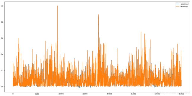
plt.plot(yhat,label='prodicted')
plt.plot(test_y,label="observed")
plt.show()

# invert scaling for forecast
inv_yhat = np.concatenate((yhat, test_X[:, 1:]), axis=1)
inv_yhat = scaler.inverse_transform(inv_yhat) #反转就是反归一化,做数据还原。
inv_yhat = inv_yhat[:,0]
# invert scaling for actual
test_y = test_y.reshape((len(test_y), 1))
inv_y = np.concatenate((test_y, test_X[:, 1:]), axis=1)
inv_y = scaler.inverse_transform(inv_y)
inv_y = inv_y[:,0]
# calculate RMSE
rmse = np.sqrt(mean_squared_error(inv_y, inv_yhat))
print('Test RMSE: %.3f' % rmse)

#反归一化后的数据(怎么做得拆分,怎么在还原回去)
plt.figure(figsize=(30,20))
plt.plot(inv_yhat,label='prodicted')
plt.plot(inv_y,label="observed")
plt.show()

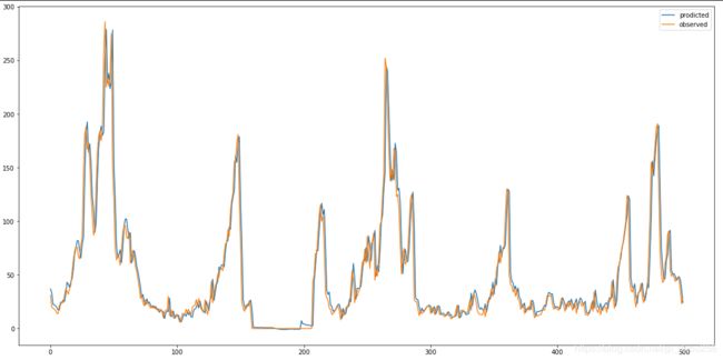
#反归一化后的数据(选取前面的500行测试数据做展示)
plt.figure(figsize=(20,10))
plt.plot(inv_yhat[:500],label='prodicted')
plt.plot(inv_y[:500],label="observed")
plt.legend()
plt.show()

数据归一化时预测的测试集数据走势效果

数据反归一化时预测的测试集数据走势效果

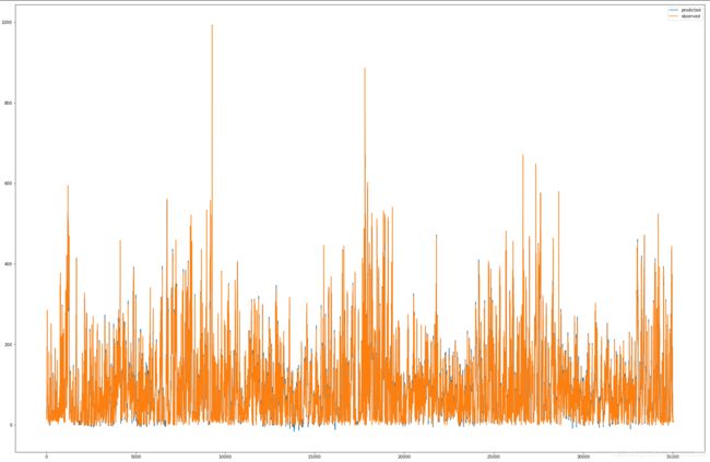
注：由于数据过多，比较密集，并没有很好地走势展示，这里仅展示前500测试条数据

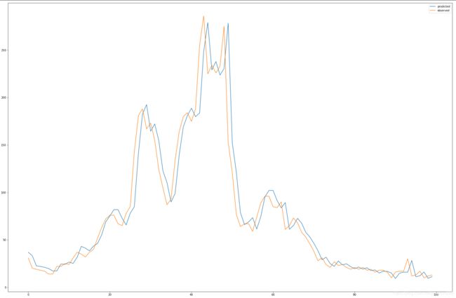
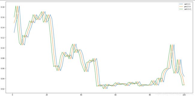
reframed = series_to_supervised(scaled, 1, 2)      #预测多各变量，取定某个变量研究过去、现在和未来的三线走势。
plt.figure(figsize=(20,10))
plt.plot(reframed['var1(t-1)'][:100],label="vart-t-1")
plt.plot(reframed['pm2.51(t)'][:100],label="pm2.5-t")
plt.plot(reframed['var1(t+1)'][:100],label="vart-t+1")
plt.legend()
plt.show()

参考博客

1. https://blog.csdn.net/fy_eng/article/details/81366723

2. 时间序列处理的函数:shift,series_to_supervised(多变量和单变量预测问题转为监督学习方式)
   https://machinelearningmastery.com/convert-time-series-supervised-learning-problem-python/

3. 平稳序列和非平稳序列概念解释和图示
   https://blog.csdn.net/zyxhangiian123456789/article/details/87458140

4.关于日期格式的转换参考博客：
https://www.jianshu.com/p/96ea42c58abe
https://blog.csdn.net/tcy23456/article/details/85292925
https://blog.csdn.net/qq_18433441/article/details/56664505