轻量级网络--MobileNet、Shufflenet

原文地址： https://blog.csdn.net/u011974639/article/details/79199306
https://blog.csdn.net/u011974639/article/details/79200559

MobileNets: Efficient Convolutional Neural Networks for Mobile Vision Applications

原文地址：MobileNetV1

代码:

• TensorFlow官方
• github-Tensorflow
• github-Caffe

---

Abstract

MobileNets是为移动和嵌入式设备提出的高效模型。MobileNets基于流线型架构(streamlined)，使用深度可分离卷积(depthwise separable convolutions,即Xception变体结构)来构建轻量级深度神经网络。

论文介绍了两个简单的全局超参数，可有效的在延迟和准确率之间做折中。这些超参数允许我们依据约束条件选择合适大小的模型。论文测试在多个参数量下做了广泛的实验，并在ImageNet分类任务上与其他先进模型做了对比，显示了强大的性能。论文验证了模型在其他领域(对象检测，人脸识别，大规模地理定位等)使用的有效性。

---

Introduction

深度卷积神经网络将多个计算机视觉任务性能提升到了一个新高度，总体的趋势是为了达到更高的准确性构建了更深更复杂的网络，但是这些网络在尺度和速度上不一定满足移动设备要求。MobileNet描述了一个高效的网络架构，允许通过两个超参数直接构建非常小、低延迟、易满足嵌入式设备要求的模型。

---

Related Work

现阶段，在建立小型高效的神经网络工作中，通常可分为两类工作：

• **压缩预训练模型。**获得小型网络的一个办法是减小、分解或压缩预训练网络，例如量化压缩(product quantization)、哈希(hashing )、剪枝(pruning)、矢量编码( vector quantization)和霍夫曼编码(Huffman coding)等；此外还有各种分解因子(various factorizations )用来加速预训练网络；还有一种训练小型网络的方法叫蒸馏(distillation )，使用大型网络指导小型网络，这是对论文的方法做了一个补充，后续有介绍补充。

• 直接训练小型模型。 例如Flattened networks利用完全的因式分解的卷积网络构建模型，显示出完全分解网络的潜力；Factorized Networks引入了类似的分解卷积以及拓扑连接的使用；Xception network显示了如何扩展深度可分离卷积到Inception V3 networks；Squeezenet 使用一个bottleneck用于构建小型网络。

本文提出的MobileNet网络架构，允许模型开发人员专门选择与其资源限制(延迟、大小)匹配的小型模型，MobileNets主要注重于优化延迟同时考虑小型网络，从深度可分离卷积的角度重新构建模型。

---

Architecture

Depthwise Separable Convolution

MobileNet是基于深度可分离卷积的。通俗的来说，深度可分离卷积干的活是：把标准卷积分解成深度卷积(depthwise convolution)和逐点卷积(pointwise convolution)。这么做的好处是可以大幅度降低参数量和计算量。分解过程示意图如下：

输入的特征映射$FFF$尺寸为$(DF,DF,M)(D_F,D_F,M)(DF,DF,M)$，采用的标准卷积$KKK$为$(DK,DK,M,N)(D_K,D_K,M,N)(DK,DK,M,N)$(如图(a)所示)，输出的特征映射为$GGG$尺寸为$(DG,DG,N)(D_G,D_G,N)(DG,DG,N)$

标准卷积的卷积计算公式为：$$Gk,l,n=\sum i,j,mKi,j,m,n\cdot Fk+i-1,l+j-1,m{G}_{k,l,n}=\sum _{i,j,m}{K}_{i,j,m,n}\cdot F_{k+i-1,l+j-1,m}Gk,l,n=i,j,m\sum Ki,j,m,n\cdot Fk+i-1,l+j-1,m$$ 输入的通道数为$MMM$,输出的通道数为$NNN$。对应的计算量为：$DK\cdot DK\cdot M\cdot N\cdot DF\cdot DF{D}_K\cdot D_K\cdot M\cdot N\cdot D_F\cdot D_{F}DK\cdot DK\cdot M\cdot N\cdot DF\cdot DF$

可将标准卷积$(DK,DK,M,N)(D_K,D_K,M,N)(DK,DK,M,N)$拆分为深度卷积和逐点卷积：

• 深度卷积负责滤波作用,尺寸为$(DK,DK,1,M)(D_K,D_K,1,M)(DK,DK,1,M)$如图(b)所示。输出特征为$(DG,DG,M)(D_G,D_G,M)(DG,DG,M)$
• 逐点卷积负责转换通道，尺寸为$(1,1,M,N)(1,1,M,N)(1,1,M,N)$如图©所示。得到最终输出为$(DG,DG,N)(D_G,D_G,N)(DG,DG,N)$

深度卷积的卷积公式为：$$G^k,l,n=\sum i,j{K}^i,j,m\cdot Fk+i-1,l+j-1,m{\hat{G}}_{k,l,n}=\sum _{i,j}{\hat{K}}_{i,j,m}\cdot F_{k+i-1,l+j-1,m}{G}^k,l,n=i,j\sum K^i,j,m\cdot Fk+i-1,l+j-1,m$$其中KaTeX parse error: Got function '\hat' with no arguments as superscript at position 2: K^̲\hat{K}K^是深度卷积，卷积核为$(DK,DK,1,M)(D_K,D_K,1,M)(DK,DK,1,M)$，其中$mth{m}_{th}mth$个卷积核应用在$FFF$中第$mth{m}_{th}mth$个通道上，产生KaTeX parse error: Got function '\hat' with no arguments as superscript at position 2: G^̲\hat{G}G^上第$mth{m}_{th}mth$个通道输出.

深度卷积和逐点卷积计算量：$D_K·D_K·M·D_F·D_F + M·N·D_F·D_F $

计算量减少了:$$DK\cdot DK\cdot M\cdot DF\cdot DF+M\cdot N\cdot DF\cdot DFDK\cdot DK\cdot M\cdot N\cdot DF\cdot DF=1N+1DK2\frac{D_K\cdot D_K\cdot M\cdot D_F\cdot D_F+M\cdot N\cdot D_F\cdot D_F}{D_K\cdot D_K\cdot M\cdot N\cdot D_F\cdot D_F}=\frac{1}{N}+\frac{1}{D_K^2}DK\cdot DK\cdot M\cdot N\cdot DF\cdot DFDK\cdot DK\cdot M\cdot DF\cdot DF+M\cdot N\cdot DF\cdot DF=N1+DK21$$

深度分类卷积示例

输入图片的大小为$(6,6,3)(6,6,3)(6,6,3)$，原卷积操作是用$(4,4,3,5)(4,4,3,5)(4,4,3,5)$的卷积($4\times 44\times 44\times 4$是卷积核大小，3是卷积核通道数，5个卷积核数量)，stride=1,无padding。输出的特征尺寸为$6-41+1=3\frac{6-4}{1}+1=316-4+1=3$，即输出的特征映射为$(3,3,5)(3,3,5)(3,3,5)$

将标准卷积中选取序号为$nnn$的卷积核，大小为$(4,4,3)(4,4,3)(4,4,3)$，标准卷积过程示意图如下(注意省略了偏置单元)：

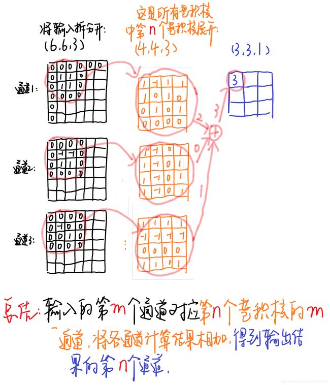
黑色的输入为$(6,6,3)(6,6,3)(6,6,3)$与第$nnn$个卷积核对应，每个通道对应每个卷积核通道卷积得到输出，最终输出为$2+0+1=32+0+1=32+0+1=3$。(这是常见的卷积操作，注意这里卷积核要和输入的通道数相同，即图中表示的3个通道~)

对于深度分离卷积，把标准卷积$(4,4,3,5)(4,4,3,5)(4,4,3,5)$分解为：

• 深度卷积部分：大小为$(4,4,1,3)(4,4,1,3)(4,4,1,3)$，作用在输入的每个通道上，输出特征映射为$(3,3,3)(3,3,3)(3,3,3)$
• 逐点卷积部分：大小为$(1,1,3,5)(1,1,3,5)(1,1,3,5)$，作用在深度卷积的输出特征映射上，得到最终输出为$(3,3,5)(3,3,5)(3,3,5)$

例中深度卷积卷积过程示意图如下：

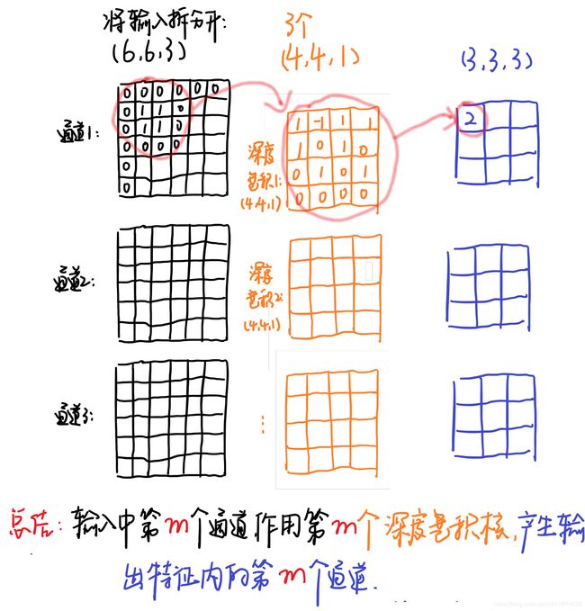
输入有3个通道，对应着有3个大小为$(4,4,1)(4,4,1)(4,4,1)$的深度卷积核，卷积结果共有3个大小为$(3,3,1)(3,3,1)(3,3,1)$，我们按顺序将这卷积按通道排列得到输出卷积结果$(3,3,3)(3,3,3)(3,3,3)$。

相比之下计算量减少了:
$4\times 4\times 3\times 54\times 4\times 3\times 54\times 4\times 3\times 5$转为了$4\times 4\times 1\times 3+1\times 1\times 3\times 54\times 4\times 1\times 3+1\times 1\times 3\times 54\times 4\times 1\times 3+1\times 1\times 3\times 5$,即参数量减少了$$4\times 4\times 1\times 3+1\times 1\times 3\times 54\times 4\times 3\times 5=2180即(15+142)\frac{4\times 4\times 1\times 3+1\times 1\times 3\times 5}{4\times 4\times 3\times 5}=\frac{21}{80}即(\frac{1}{5}+\frac{1}{4^2})4\times 4\times 3\times 54\times 4\times 1\times 3+1\times 1\times 3\times 5=8021即(51+421)$$

MobileNet使用可分离卷积减少了8到9倍的计算量，只损失了一点准确度。

Network Structure and Training

标准卷积和MobileNet中使用的深度分离卷积结构对比如下:

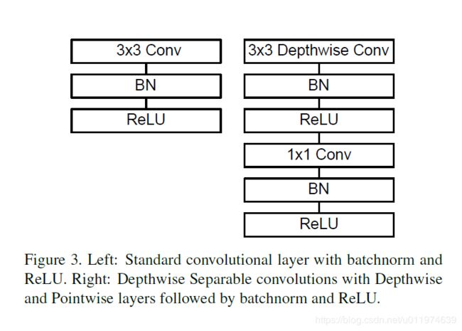
注意：如果是需要下采样，则在第一个深度卷积上取步长为2.

MobileNet的具体结构如下(dw表示深度分离卷积)：

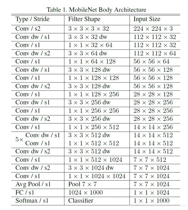
除了最后的FC层没有非线性激活函数，其他层都有BN和ReLU非线性函数.

我们的模型几乎将所有的密集运算放到$1\times 11\times 11\times 1$卷积上，这可以使用general matrix multiply (GEMM) functions优化。在MobileNet中有95%的时间花费在$1\times 11\times 11\times 1$卷积上,这部分也占了75%的参数：

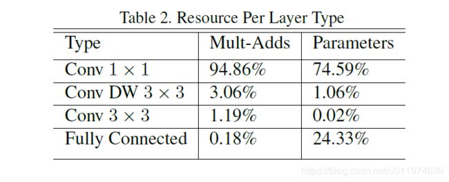
剩余的其他参数几乎都在FC层上了。

在TensorFlow中使用RMSprop对MobileNet做训练，使用类似InceptionV3 的异步梯度下降。与训练大型模型不同的是，我们较少使用正则和数据增强技术，因为小模型不易陷入过拟合；没有使用side heads or label smoothing，我们发现在深度卷积核上放入很少的L2正则或不设置权重衰减的很重要，因为这部分参数很少。

Width Multiplier: Thinner Models

我们引入的第一个控制模型大小的超参数是：宽度因子$\alpha \alpha \alpha$(Width multiplier )，用于控制输入和输出的通道数，即输入通道从$MMM$变为$\alpha M\alpha M\alpha M$,输出通道从$NNN$变为$\alpha N\alpha N\alpha N$。

深度卷积和逐点卷积的计算量：$$DK\cdot DK\cdot \alpha M\cdot DF\cdot DF+\alpha M\cdot \alpha N\cdot DF\cdot DF{D}_K\cdot D_K\cdot \alpha M\cdot D_F\cdot D_F+\alpha M\cdot \alpha N\cdot D_F\cdot D_{F}DK\cdot DK\cdot \alpha M\cdot DF\cdot DF+\alpha M\cdot \alpha N\cdot DF\cdot DF$$可设置$\alpha \in (0,1]\alpha \in (0,1]\alpha \in (0,1]$，通常取$1,0.75,0.5和0.251,0.75,0.5和0.251,0.75,0.5和0.25$。

计算量减少了:$$DK\cdot DK\cdot \alpha M\cdot DF\cdot DF+\alpha M\cdot \alpha N\cdot DF\cdot DFDK\cdot DK\cdot M\cdot N\cdot DF\cdot DF=\alpha N+\alpha 2DK2\frac{D_K\cdot D_K\cdot \alpha M\cdot D_F\cdot D_F+\alpha M\cdot \alpha N\cdot D_F\cdot D_F}{D_K\cdot D_K\cdot M\cdot N\cdot D_F\cdot D_F}=\frac{\alpha }{N}+\frac{{\alpha }^2}{D_K^2}DK\cdot DK\cdot M\cdot N\cdot DF\cdot DFDK\cdot DK\cdot \alpha M\cdot DF\cdot DF+\alpha M\cdot \alpha N\cdot DF\cdot DF=N\alpha +DK2\alpha 2$$

宽度因子将计算量和参数降低了约$\alpha 2{\alpha }^2\alpha 2$倍，可很方便的控制模型大小.

Resolution Multiplier: Reduced Representation

我们引入的第二个控制模型大小的超参数是：分辨率因子$\rho \rho \rho$(resolution multiplier ).用于控制输入和内部层表示。即用分辨率因子控制输入的分辨率。

深度卷积和逐点卷积的计算量：$$DK\cdot DK\cdot \alpha M\cdot \rho DF\cdot \rho DF+\alpha M\cdot \alpha N\cdot \rho DF\cdot \rho DF{D}_K\cdot D_K\cdot \alpha M\cdot \rho D_F\cdot \rho D_F+\alpha M\cdot \alpha N\cdot \rho D_F\cdot \rho D_{F}DK\cdot DK\cdot \alpha M\cdot \rho DF\cdot \rho DF+\alpha M\cdot \alpha N\cdot \rho DF\cdot \rho DF$$可设置$\rho \in (0,1]\rho \in (0,1]\rho \in (0,1]$，通常设置输入分辨率为$224,192,160和128224,192,160和128224,192,160和128$。

计算量减少了:$$DK\cdot DK\cdot \alpha M\cdot \rho DF\cdot \rho DF+\alpha M\cdot \alpha N\cdot \rho DF\cdot \rho DFDK\cdot DK\cdot M\cdot N\cdot DF\cdot DF=\alpha \rho N+\alpha 2\rho 2DK2\frac{D_K\cdot D_K\cdot \alpha M\cdot \rho D_F\cdot \rho D_F+\alpha M\cdot \alpha N\cdot \rho D_F\cdot \rho D_F}{D_K\cdot D_K\cdot M\cdot N\cdot D_F\cdot D_F}=\frac{\alpha \rho }{N}+\frac{{\alpha }^2{\rho }^2}{D_K^2}DK\cdot DK\cdot M\cdot N\cdot DF\cdot DFDK\cdot DK\cdot \alpha M\cdot \rho DF\cdot \rho DF+\alpha M\cdot \alpha N\cdot \rho DF\cdot \rho DF=N\alpha \rho +DK2\alpha 2\rho 2$$

分辨率因子将计算量和参数降低了约$\rho 2{\rho }^2\rho 2$倍，可很方便的控制模型大小.

下面的示例展现了宽度因子和分辨率因子对模型的影响：

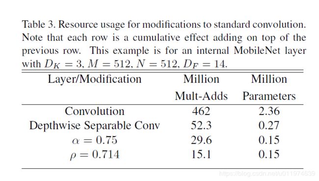
第一行是使用标准卷积的参数量和Mult-Adds；第二行将标准卷积改为深度分类卷积，参数量降低到约为原本的1/10，Mult-Adds降低约为原本的1/9。使用$\alpha 和\rho \alpha 和\rho \alpha 和\rho$参数可以再将参数降低一半，Mult-Adds再成倍下降。

---

Experiment

实验部分主要研究以下部分： 深度卷积的影响；宽度因子的影响；两个超参数的权衡；与其他模型对比。

Model Choices

使用深度分类卷积的MobileNet与使用标准卷积的MobileNet之间对比：

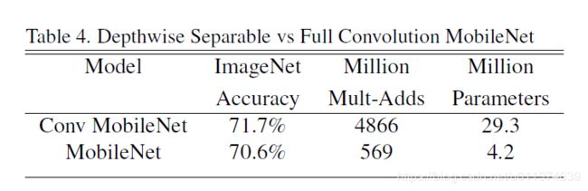
在精度上损失了1%，但是的计算量和参数量上降低了一个数量级。

原MobileNet的配置如下：

为了进一步缩小模型，可将MobileNet中的5层$14\times 14\times 51214\times 14\times 51214\times 14\times 512$的深度可分离卷积去除。

实验结果对比：

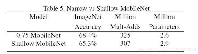
可以看到在类似的参数量和计算量下，精度衰减了3%。(中间的深度卷积用于过滤作用，参数量少，冗余度相比于大量的逐点卷积应该是少很多的~)

Model Shrinking Hyperparameters

单参数验证

表6显示宽度因子对模型参数量、计算量精度的影响，表7显示分辨率因子对模型参数量、计算量精度的影响：

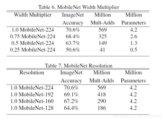
使用过程要权衡参数对模型性能和大小的影响。

交叉验证计算量对精度影响

图4显示了16个交叉的模型在ImageNet上的表现，宽度因子取值为$\alpha \in 1,0.75,0.5,0.25\alpha \in \{1,0.75,0.5,0.25\}\alpha \in 1,0.75,0.5,0.25$，分辨率取值为$224,192,160,128\{224,192,160,128\}224,192,160,128$。

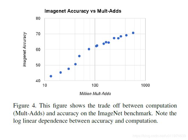
当模型越来越小时，精度可近似看成对数跳跃形式的。

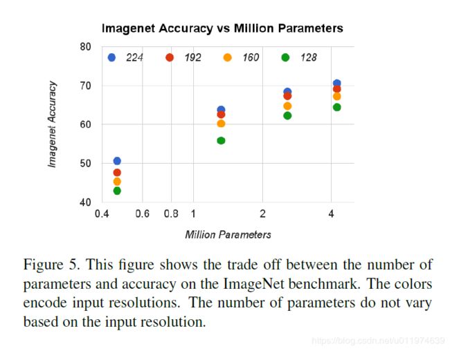
交叉验证参数量对精度影响

图5显示了16个交叉的模型在ImageNet上的表现，宽度因子取值为$\alpha \in 1,0.75,0.5,0.25\alpha \in \{1,0.75,0.5,0.25\}\alpha \in 1,0.75,0.5,0.25$，分辨率取值为$224,192,160,128\{224,192,160,128\}224,192,160,128$。

与其他先进模型相比

表8将完整的MobileNet与原始的GoogleNet和VGG16对比，MobileNet与VGG16有相似的精度，参数量和计算量减少了2个数量级。

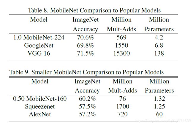
表9是MobileNet的宽度因子$\alpha =0.5\alpha =0.5\alpha =0.5$和分辨率设置为$160\times 160160\times 160160\times 160$的缩小模型与其他模型对比结果，相比于老大哥AlexNet在计算量和参数量上都降低一个数量级，对比同为小型网络的Squeezenet，计算量少了2个数量级，在参数量类似的情况下，精度高了3%。

其他应用场景性能

Fine Grained Recognition

在Stanford Dogs dataset的表现如下：

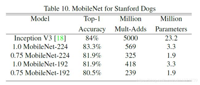
MobileNet在计算量和参数量降低一个数量级的同时几乎保持相同的精度。

Large Scale Geolocalizaton

PlaNet是做大规模地理分类任务，我们使用MobileNet的框架重新设计了PlaNet，对比如下：

基于Inception V3架构的PlaNet有5200万参数和574亿的mult-adds，而基于MobileNet的PlaNet只有1300万参数(300个是主体参数，1000万是最后分类层参数)和58万的mult-adds，相比之下，只是性能稍微受损，但还是比原Im2GPS效果好多了。

Face Attributes

MobileNet的框架技术可用于压缩大型模型，在Face Attributes任务中，我们验证了MobileNet的蒸馏(distillation )技术的关系，蒸馏的核心是让小模型去模拟大模型，而不是直接逼近Ground Label：

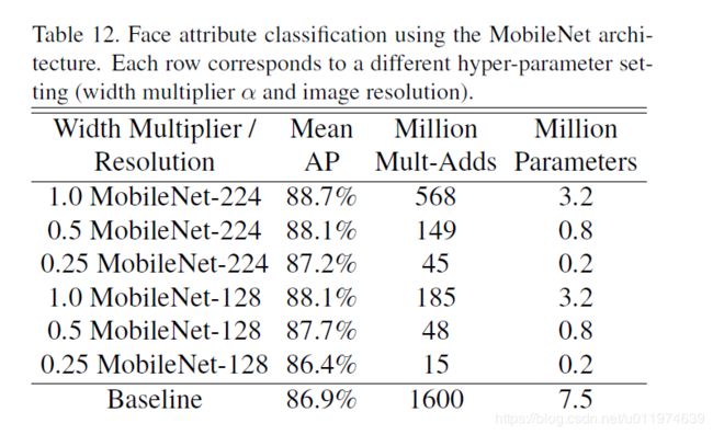
将蒸馏技术的可扩展性和MobileNet技术的精简性结合到一起，最终系统不仅不需要正则技术(例如权重衰减和退火等)，而且表现出更强的性能。

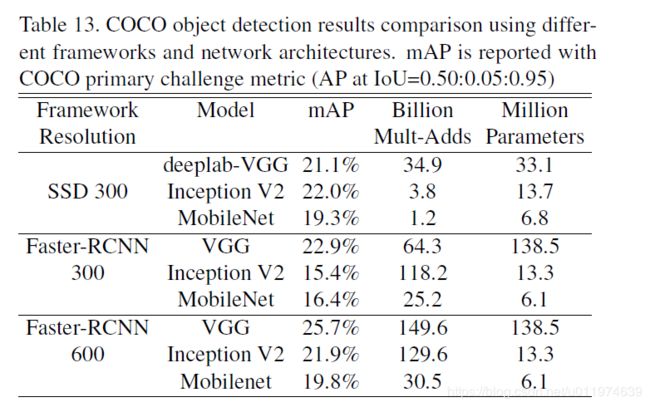
Object Detection

基于MobileNet改进的检测模型对比如下：

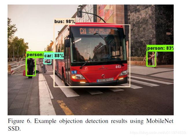
可视化结果：

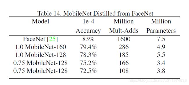
Face Embeddings

FaceNet是现阶段最先进的人脸识别模型，基于MobileNet和蒸馏技术训练出结果如下：

---

Conclusion

论文提出了一种基于深度可分离卷积的新模型MobileNet，同时提出了两个超参数用于快速调节模型适配到特定环境。实验部分将MobileNet与许多先进模型做对比，展现出MobileNet的在尺寸、计算量、速度上的优越性。

---

代码分析

这里参考的代码是mobilenet.py文件（当然也可以参考TensoeFlow官方的MobileNet）

TensorFlow有实现好的深度卷积API，所以整个代码非常整洁的~

具体的API参考tf.contrib.layers.separable_conv2d文档~

'''
100% Mobilenet V1 (base) with input size 224x224:
See mobilenet_v1()
Layer                                                     params           macs
--------------------------------------------------------------------------------
MobilenetV1/Conv2d_0/Conv2D:                                 864      10,838,016
MobilenetV1/Conv2d_1_depthwise/depthwise:                    288       3,612,672
MobilenetV1/Conv2d_1_pointwise/Conv2D:                     2,048      25,690,112
MobilenetV1/Conv2d_2_depthwise/depthwise:                    576       1,806,336
MobilenetV1/Conv2d_2_pointwise/Conv2D:                     8,192      25,690,112
MobilenetV1/Conv2d_3_depthwise/depthwise:                  1,152       3,612,672
MobilenetV1/Conv2d_3_pointwise/Conv2D:                    16,384      51,380,224
MobilenetV1/Conv2d_4_depthwise/depthwise:                  1,152         903,168
MobilenetV1/Conv2d_4_pointwise/Conv2D:                    32,768      25,690,112
MobilenetV1/Conv2d_5_depthwise/depthwise:                  2,304       1,806,336
MobilenetV1/Conv2d_5_pointwise/Conv2D:                    65,536      51,380,224
MobilenetV1/Conv2d_6_depthwise/depthwise:                  2,304         451,584
MobilenetV1/Conv2d_6_pointwise/Conv2D:                   131,072      25,690,112
MobilenetV1/Conv2d_7_depthwise/depthwise:                  4,608         903,168
MobilenetV1/Conv2d_7_pointwise/Conv2D:                   262,144      51,380,224
MobilenetV1/Conv2d_8_depthwise/depthwise:                  4,608         903,168
MobilenetV1/Conv2d_8_pointwise/Conv2D:                   262,144      51,380,224
MobilenetV1/Conv2d_9_depthwise/depthwise:                  4,608         903,168
MobilenetV1/Conv2d_9_pointwise/Conv2D:                   262,144      51,380,224
MobilenetV1/Conv2d_10_depthwise/depthwise:                 4,608         903,168
MobilenetV1/Conv2d_10_pointwise/Conv2D:                  262,144      51,380,224
MobilenetV1/Conv2d_11_depthwise/depthwise:                 4,608         903,168
MobilenetV1/Conv2d_11_pointwise/Conv2D:                  262,144      51,380,224
MobilenetV1/Conv2d_12_depthwise/depthwise:                 4,608         225,792
MobilenetV1/Conv2d_12_pointwise/Conv2D:                  524,288      25,690,112
MobilenetV1/Conv2d_13_depthwise/depthwise:                 9,216         451,584
MobilenetV1/Conv2d_13_pointwise/Conv2D:                1,048,576      51,380,224
--------------------------------------------------------------------------------
Total:                                                 3,185,088     567,716,352
'''

def mobilenet(inputs,
num_classes=1000,
is_training=True,
width_multiplier=1,
scope=‘MobileNet’):
“”" MobileNet
More detail, please refer to Google’s paper(https://arxiv.org/abs/1704.04861).

Args:
inputs: a tensor of size [batch_size, height, width, channels].
num_classes: number of predicted classes.
is_training: whether or not the model is being trained.
scope: Optional scope for the variables.
Returns:
logits: the pre-softmax activations, a tensor of size
[batch_size, num_classes]
end_points: a dictionary from components of the network to the corresponding
activation.
“”"
# depthwise_separable_conv内包含深度卷积和逐点卷积
def _depthwise_separable_conv(inputs,
num_pwc_filters,
width_multiplier,
sc,
downsample=False):
“”" Helper function to build the depth-wise separable convolution layer.
“”"
num_pwc_filters = round(num_pwc_filters * width_multiplier)
_stride = 2 if downsample else 1

# 设置num_outputs=None跳过逐点卷积
depthwise_conv = slim.separable_convolution2d(inputs,
num_outputs=None,
stride=_stride,
depth_multiplier=1,
kernel_size=[3, 3],
scope=sc+’/depthwise_conv’)

bn = slim.batch_norm(depthwise_conv, scope=sc+’/dw_batch_norm’)
# 逐点卷积变换通道
pointwise_conv = slim.convolution2d(bn,
num_pwc_filters,
kernel_size=[1, 1],
scope=sc+’/pointwise_conv’)
bn = slim.batch_norm(pointwise_conv, scope=sc+’/pw_batch_norm’)
return bn

with tf.variable_scope(scope) as sc:
end_points_collection = sc.name + ‘_end_points’
with slim.arg_scope([slim.convolution2d, slim.separable_convolution2d],
activation_fn=None,
outputs_collections=[end_points_collection]):
with slim.arg_scope([slim.batch_norm],
is_training=is_training,
activation_fn=tf.nn.relu,
fused=True):

# 定义整体结构
net = slim.convolution2d(inputs, round(32 * width_multiplier), [3, 3], stride=2, padding=‘SAME’, scope=‘conv_1’)
net = slim.batch_norm(net, scope=‘conv_1/batch_norm’)
net = _depthwise_separable_conv(net, 64, width_multiplier, sc=‘conv_ds_2’)
net = _depthwise_separable_conv(net, 128, width_multiplier, downsample=True, sc=‘conv_ds_3’)
net = _depthwise_separable_conv(net, 128, width_multiplier, sc=‘conv_ds_4’)
net = _depthwise_separable_conv(net, 256, width_multiplier, downsample=True, sc=‘conv_ds_5’)
net = _depthwise_separable_conv(net, 256, width_multiplier, sc=‘conv_ds_6’)
net = _depthwise_separable_conv(net, 512, width_multiplier, downsample=True, sc=‘conv_ds_7’)

net = _depthwise_separable_conv(net, 512, width_multiplier, sc=‘conv_ds_8’)
net = _depthwise_separable_conv(net, 512, width_multiplier, sc=‘conv_ds_9’)
net = _depthwise_separable_conv(net, 512, width_multiplier, sc=‘conv_ds_10’)
net = _depthwise_separable_conv(net, 512, width_multiplier, sc=‘conv_ds_11’)
net = _depthwise_separable_conv(net, 512, width_multiplier, sc=‘conv_ds_12’)
net = _depthwise_separable_conv(net, 1024, width_multiplier, downsample=True, sc=‘conv_ds_13’)
net = _depthwise_separable_conv(net, 1024, width_multiplier, sc=‘conv_ds_14’)
net = slim.avg_pool2d(net, [7, 7], scope=‘avg_pool_15’)
end_points = slim.utils.convert_collection_to_dict(end_points_collection)
net = tf.squeeze(net, [1, 2], name=‘SpatialSqueeze’)
end_points[‘squeeze’] = net

# 接FC再接Softmax
logits = slim.fully_connected(net, num_classes, activation_fn=None, scope=‘fc_16’)
predictions = slim.softmax(logits, scope=‘Predictions’)

end_points[‘Logits’] = logits
end_points[‘Predictions’] = predictions

return logits, end_points

mobilenet.default_image_size = 224