Coursera-吴恩达-机器学习-第五周-编程作业: Neural Networks Learning
本次文章内容: Coursera吴恩达机器学习课程,第五周编程作业。编程语言是Matlab。
学习算法分两部分进行理解,第一部分是根据code对算法进行综述,第二部分是代码。
0 Introduction
在这个练习中,将应用 backpropagation,实现神经网络来识别手写数字。
1 Neural Networks
Algorithm
Part 0 Initialization & Setup the parameters
clear ; close all; clc 的三剑客常规操作。并设置神经网络的结构参数。
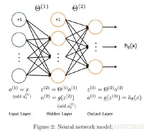
下图是我们的Model representation:一共是三层,an input layer,a hidden layer and an output layer.
Part 1: Loading and Visualizing Data
随机选取100个data进行可视化。
Part 2: Loading Parameters
加载已经训练好的theta参数,并将theta展开为我们需要的向量形式。
Part 3: Compute Cost (Feedforward)
要做back propagation,先要做feedforward得到每个class的hypothesis。这部分的代码主要整合在 nnCostFunction()函数中。 根据我们的model,计算得到每个note的activation值,计算cost function(带正则项)。next,我们会在这个函数里计算back propagation,从后向前计算detla value,then计算累积误差,then计算cost function的partial derivative(带正则项)。
Part 4: Implement Regularization
刚刚说到了,并输入测试值检测是否得出正确值。
Part 5: Sigmoid Gradient
sigmoid 函数的derivative有个特殊性质,这里计算其导数。
Part 6: Initializing Pameters
为了防止所有的theta的初始值都是零,或者same,这将会倒是 back propagation 的计算无意义。所以我们random initialization ,根据维度rand() 0或1 value。
Part 7: Implement Backpropagation
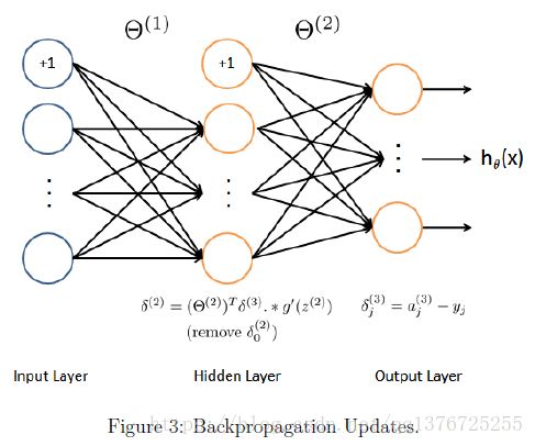
按4步,计算cost function的gradient,
1. 计算forward propagation,computing the activations for all layers,注意bias的 +1term。
2.从output开始从后往前计算detla值
3.计算hidden layer 的detla 值,注意skip 第一层的detla 值
4.Accumulate all the gradient值
5. Obtain the (unregularized) gradient for cost function。
注意,只有 成功  completed the feedforward之后,才可以implementing the backpropagation algorithm,
Part 8: Implement Regularization
上一步中,添加正则项,在求cost function的gradient得第五步时。
Part 8: Training NN
在我们获得了cost和gradient之后,我们可以通过fmincg()函数来train neural network。
Part 9: Visualize Weights
对中间层的像素,进行可视化。
Part 10: Implement Predict
After training the neural network,我们 计算 training set accuracy。
Code
下面是nnCostFunction()函数部分,其他部分难度不大。
function [J grad] = nnCostFunction(nn_params, ...
                                   input_layer_size, ...
                                   hidden_layer_size, ...
                                   num_labels, ...
                                   X, y, lambda)
%NNCOSTFUNCTION Implements the neural network cost function for a two layer
%neural network which performs classification
%   [J grad] = NNCOSTFUNCTON(nn_params, hidden_layer_size, num_labels, ...
%   X, y, lambda) computes the cost and gradient of the neural network. The
%   parameters for the neural network are "unrolled" into the vector
%   nn_params and need to be converted back into the weight matrices.
%
%   The returned parameter grad should be a "unrolled" vector of the
%   partial derivatives of the neural network.
%

% Reshape nn_params back into the parameters Theta1 and Theta2, the weight matrices
% for our 2 layer neural network
Theta1 = reshape(nn_params(1:hidden_layer_size * (input_layer_size + 1)), ...
                 hidden_layer_size, (input_layer_size + 1));

Theta2 = reshape(nn_params((1 + (hidden_layer_size * (input_layer_size + 1))):end), ...
                 num_labels, (hidden_layer_size + 1));

% Setup some useful variables
m = size(X, 1);

% You need to return the following variables correctly
J = 0;
Theta1_grad = zeros(size(Theta1));
Theta2_grad = zeros(size(Theta2));

% ====================== YOUR CODE HERE ======================
% Instructions: You should complete the code by working through the
%               following parts.
%
% Part 1: Feedforward the neural network and return the cost in the
%         variable J. After implementing Part 1, you can verify that your
%         cost function computation is correct by verifying the cost
%         computed in ex4.m
%
% Part 2: Implement the backpropagation algorithm to compute the gradients
%         Theta1_grad and Theta2_grad. You should return the partial derivatives of
%         the cost function with respect to Theta1 and Theta2 in Theta1_grad and
%         Theta2_grad, respectively. After implementing Part 2, you can check
%         that your implementation is correct by running checkNNGradients
%
%         Note: The vector y passed into the function is a vector of labels
%               containing values from 1..K. You need to map this vector into a
%               binary vector of 1's and 0's to be used with the neural network
%               cost function.
%
%         Hint: We recommend implementing backpropagation using a for-loop
%               over the training examples if you are implementing it for the
%               first time.
%
% Part 3: Implement regularization with the cost function and gradients.
%
%         Hint: You can implement this around the code for
%               backpropagation. That is, you can compute the gradients for
%               the regularization separately and then add them to Theta1_grad
%               and Theta2_grad from Part 2.
%

%me******************************************************
%X= [ones(m,1)  X];
%a1 = sigmoid(X * Theta1');

%m1 = size(a1 ,1);
%X1 = [ones(m1,1) a1];
%hx = sigmoid(X1 * Theta2');

%[p pp] = max(hx, [], 1);
%J1 = (-y).* log(pp) - (1-y).* log(1-pp);
%J = 1/m * sum(J1);

%deta1 = pp -y;
%teacher&***********************************************

ylable = zeros(num_labels, m);   %10x5000
for i = 1:m
    ylable(y(i),i) = 1;
end

a1 = [ones(m,1) X];    %5000x401
z2 = a1 * Theta1';     %5000x25
a2 = sigmoid(z2);

a2 = [ones(m,1) a2];      %5000x26
a3 = sigmoid(a2 * Theta2');        %5000x10


J = 1 / m * sum( sum( -ylable'.* log(a3) -  (1-ylable').*log(1-a3) ));

% pay attention :" Theta1(:,2:end) " , no "Theta1" .
regularized = lambda/(2*m) * (sum(sum(Theta1(:,2:end).^2)) + sum(sum(Theta2(:,2:end).^2)) );

J = J + regularized;

delta3 = a3-ylable';            %5000x10

delta2 = delta3 * Theta2 ;  %5000x26
delta2 = delta2(:,2:end);    %5000x25
delta2 = delta2 .* sigmoidGradient(z2);  %5000x25

Delta_1 = zeros(size(Theta1));        %25x401
Delta_2 = zeros(size(Theta2));         %10x26

Delta_1 = Delta_1 + delta2' * a1 ;    %25x401
Delta_2 = Delta_2 + delta3' * a2 ;     %10x26

Theta1_grad = 1/m * Delta_1;
Theta2_grad = 1/m * Delta_2;

% do the regularization
regularized_1 = lambda/m * Theta1;
regularized_2 = lambda/m * Theta2;
% j = 0 is not need to do the regularization
regularized_1(:,1) = zeros(size(regularized_1,1),1);
regularized_2(:,1) = zeros(size(regularized_2,1),1);

Theta1_grad = Theta1_grad + regularized_1;
Theta2_grad = Theta2_grad + regularized_2;

% -------------------------------------------------------------

% =========================================================================

% Unroll gradients
grad = [Theta1_grad(:) ; Theta2_grad(:)];


end

