目标检测 -- SSD (tensorflow 版) 逐行逐句解读
目标检测 -- SSD (tensorflow 版) 逐行逐句解读
这篇博客,主要是讲解SSD,tensorflow版的实现,代码地址是:SSD-tensorflow,大神写的代码,也是github上tensorflow版的SSD star 最多的代码,所以就用它来讲解,同时附上论文地址:SSD 论文下载
对照论文和代码讲解,代码中提供了SSD300和SSD512,代码一样,只是图像输入大小不一致,这个地方我主要讲解SSD512。
1 网络结构
我们先来看论文上的网络结构图:

网络结构比较简单,就是在VGG的基础上改得,前面和VGG一样,但是SSD把VGG的全连接层换成了几个卷积层,把droupout层去除了,同时使用了atrous algorithm,其实就是扩展卷积或带孔卷积(Dilation Conv),具体这个卷积方式可以看这个链接 atrous algorithm。
我们从图上也可以看出,SSD和YOLO不同的地方是,YOLO只是对最后一层特征图用来预测回归框,而SSD则是多层,不同大小的特征图都用来做预测和回归。YOLO的缺点是定位不准,对小物体检测效果差,而SSD一定长度上克服了这些难点,因为使用了不同特征图进行预测,SSD的多尺度,用的多层的特征图,是stride=2,不断缩小特征图的长和宽,越靠后的卷积特征图,他的感受野越大,越靠前感受野越小,同时越靠前检测小物体效果更好。但是SSD对小物体检测也并不好,因为前面VGG的已经把特征图下降了16倍。
我们看下网络结构的代码:
    end_points = {}
    with tf.variable_scope(scope, 'ssd_512_vgg', [inputs], reuse=reuse):
        # Original VGG-16 blocks.
        net = slim.repeat(inputs, 2, slim.conv2d, 64, [3, 3], scope='conv1')
        end_points['block1'] = net
        net = slim.max_pool2d(net, [2, 2], scope='pool1')
        # Block 2.
        net = slim.repeat(net, 2, slim.conv2d, 128, [3, 3], scope='conv2')
        end_points['block2'] = net
        net = slim.max_pool2d(net, [2, 2], scope='pool2')
        # Block 3.
        net = slim.repeat(net, 3, slim.conv2d, 256, [3, 3], scope='conv3')
        end_points['block3'] = net
        net = slim.max_pool2d(net, [2, 2], scope='pool3')
        # Block 4.
        net = slim.repeat(net, 3, slim.conv2d, 512, [3, 3], scope='conv4')
        end_points['block4'] = net
        net = slim.max_pool2d(net, [2, 2], scope='pool4')
        # Block 5.
        net = slim.repeat(net, 3, slim.conv2d, 512, [3, 3], scope='conv5')
        end_points['block5'] = net
        net = slim.max_pool2d(net, [3, 3], 1, scope='pool5')

        # Additional SSD blocks.
        # Block 6: let's dilate the hell out of it!
        net = slim.conv2d(net, 1024, [3, 3], rate=6, scope='conv6')
        end_points['block6'] = net
        # Block 7: 1x1 conv. Because the fuck.
        net = slim.conv2d(net, 1024, [1, 1], scope='conv7')
        end_points['block7'] = net

        # Block 8/9/10/11: 1x1 and 3x3 convolutions stride 2 (except lasts).
        end_point = 'block8'
        with tf.variable_scope(end_point):
            net = slim.conv2d(net, 256, [1, 1], scope='conv1x1')
            net = custom_layers.pad2d(net, pad=(1, 1))
            net = slim.conv2d(net, 512, [3, 3], stride=2, scope='conv3x3', padding='VALID')
        end_points[end_point] = net
        end_point = 'block9'
        with tf.variable_scope(end_point):
            net = slim.conv2d(net, 128, [1, 1], scope='conv1x1')
            net = custom_layers.pad2d(net, pad=(1, 1))
            net = slim.conv2d(net, 256, [3, 3], stride=2, scope='conv3x3', padding='VALID')
        end_points[end_point] = net
        end_point = 'block10'
        with tf.variable_scope(end_point):
            net = slim.conv2d(net, 128, [1, 1], scope='conv1x1')
            net = custom_layers.pad2d(net, pad=(1, 1))
            net = slim.conv2d(net, 256, [3, 3], stride=2, scope='conv3x3', padding='VALID')
        end_points[end_point] = net
        end_point = 'block11'
        with tf.variable_scope(end_point):
            net = slim.conv2d(net, 128, [1, 1], scope='conv1x1')
            net = custom_layers.pad2d(net, pad=(1, 1))
            net = slim.conv2d(net, 256, [3, 3], stride=2, scope='conv3x3', padding='VALID')
        end_points[end_point] = net
        end_point = 'block12'
        with tf.variable_scope(end_point):
            net = slim.conv2d(net, 128, [1, 1], scope='conv1x1')
            net = custom_layers.pad2d(net, pad=(1, 1))
            net = slim.conv2d(net, 256, [4, 4], scope='conv4x4', padding='VALID')
            # Fix padding to match Caffe version (pad=1).
            # pad_shape = [(i-j) for i, j in zip(layer_shape(net), [0, 1, 1, 0])]
            # net = tf.slice(net, [0, 0, 0, 0], pad_shape, name='caffe_pad')
        end_points[end_point] = net

        # Prediction and localisations layers.
        predictions = []
        logits = []
        localisations = []
        for i, layer in enumerate(feat_layers):
            with tf.variable_scope(layer + '_box'):
                ## p = cls_pred,l =  loc_pred ,表示每一层的预测结果
                p, l = ssd_vgg_300.ssd_multibox_layer(end_points[layer],
                                                      num_classes,
                                                      anchor_sizes[i],
                                                      anchor_ratios[i],
                                                      normalizations[i])
            ## 对于类别在进行tf.softmax
            predictions.append(prediction_fn(p))
            logits.append(p)
            localisations.append(l)
上面的代码就是在构建网络,网络也就是和VGG差不多,endpoints这个字典,里面包含的是不同特征图的输出,就是SSD不是只利用一层特征,而是多层,所以这个地方存放多层的输出。需要注意,原本程序我把每一层的输出特征图大小都计算了,结果没保存,就是如果仔细取计算每一层的输出特征图的大小,会发现,后面有8×8,4×4大小的特征图,最后一层是1×1,这个是作者设计的,所以如果想换成其他的网络,有时我们自己也是需要设计这样的,就是代码中为啥有时候要加一个padd,就是为了保证最后输出结果为1×1,以及有类似8×8和4×4大小的特征图具体怎么算,可以看这个博客:点击打开链接
我们看几个参数:
        feat_layers=['block4', 'block7', 'block8', 'block9', 'block10', 'block11', 'block12'],
        feat_shapes=[(64, 64), (32, 32), (16, 16), (8, 8), (4, 4), (2, 2), (1, 1)],
anchor_steps=[8, 16, 32, 64, 128, 256, 512],这个几个feature -map的大小就是根据网络结构算出来的,64×64之类的,大家可以去计算,发现是对应的,block4的特征图大小就是64,所以大家想换网络,这个地方需要计算好自己改。anchor_steps也是对应的,就是特征图的缩放倍数,也是对对应的,比如:8×64=512,16×32=512等等。不能随便设置
然后上面代码中有ssd_vgg_300.ssd_multibox_layer这个函数,我们看一下:
def ssd_multibox_layer(inputs,
                       num_classes,
                       sizes,
                       ratios=[1],
                       normalization=-1,
                       bn_normalization=False):
    """Construct a multibox layer, return a class and localization predictions.
    """
    net = inputs
    if normalization > 0:
        net = custom_layers.l2_normalization(net, scaling=True)
    # Number of anchors.
    num_anchors = len(sizes) + len(ratios)

    # Location.
    num_loc_pred = num_anchors * 4
    loc_pred = slim.conv2d(net, num_loc_pred, [3, 3], activation_fn=None,
                           scope='conv_loc')
    loc_pred = custom_layers.channel_to_last(loc_pred)
    loc_pred = tf.reshape(loc_pred,
                          tensor_shape(loc_pred, 4)[:-1]+[num_anchors, 4])
    # Class prediction.
    num_cls_pred = num_anchors * num_classes
    cls_pred = slim.conv2d(net, num_cls_pred, [3, 3], activation_fn=None,
                           scope='conv_cls')
    cls_pred = custom_layers.channel_to_last(cls_pred)
    cls_pred = tf.reshape(cls_pred,
                          tensor_shape(cls_pred, 4)[:-1]+[num_anchors, num_classes])
    return cls_pred, loc_pred
上面代码中,我们对于输出特征图,直接经过3×3的卷积层输出框和类别,custom_layers.channel_to_last,这个函数其实只是把通道数放在最后,但是tensorlfow里面本来就是,所以有点多余,num_anchors表示该层框的个数。
tensor_shape(cls_pred, 4)[:-1]+[num_anchors, num_classes]tensor_shape(loc_pred, 4)[:-1]+[num_anchors, 4]tensor_shape 就是将tensor的形状拿到,然后把最后一层拆分出来,变为5维的相当于,后两两个维度代表那个框,的那个类或者框,然后返回类和框的预测,注意这个地方这两个输出都没激活函数。
然后在回到网络结构后面的代码:
        for i, layer in enumerate(feat_layers):
            with tf.variable_scope(layer + '_box'):
                ## p = cls_pred,l =  loc_pred ,表示每一层的预测结果
                p, l = ssd_vgg_300.ssd_multibox_layer(end_points[layer],
                                                      num_classes,
                                                      anchor_sizes[i],
                                                      anchor_ratios[i],
                                                      normalizations[i])
            ## 对于类别在进行tf.softmax
            predictions.append(prediction_fn(p))
            logits.append(p)
            localisations.append(l)

        return predictions, localisations, logits, end_points
这个地方就是循环,然后把结果保存在一个list中,prediction_fn就是softmax,因为前面是没有激活函数的,所以prediction是保存了经过激活函数的,logits是没有激活函数的,localisations是保存预测的框,end_poins是每一层的输出。
以上就是整个网络的架构,就是利用VGG模型,把后面的全连接层改了,全部变为卷积层,然后不是只用最后一层预测框,中间不同特征图大小都有用来预测。
2 SSD 框的生成
    def anchors(self, img_shape, dtype=np.float32):
        """Compute the default anchor boxes, given an image shape.
        """
        return ssd_anchors_all_layers(img_shape,
                                      self.params.feat_shapes,
                                      self.params.anchor_sizes,
                                      self.params.anchor_ratios,
                                      self.params.anchor_steps,
                                      self.params.anchor_offset,
                                      dtype)
代码里面框的生成实现了两连跳,这个地方入口,调用ssd_anchors_all_layers,image_shape就是图像输入大小,我们再看这个函数:
def ssd_anchors_all_layers(img_shape,
                           layers_shape,
                           anchor_sizes,
                           anchor_ratios,
                           anchor_steps,
                           offset=0.5,
                           dtype=np.float32):
    """Compute anchor boxes for all feature layers.
    """
    layers_anchors = []
    for i, s in enumerate(layers_shape):
        anchor_bboxes = ssd_anchor_one_layer(img_shape, s,
                                             anchor_sizes[i],
                                             anchor_ratios[i],
                                             anchor_steps[i],
                                             offset=offset, dtype=dtype)
        layers_anchors.append(anchor_bboxes)
    return layers_anchors
上面这个函数,是一个for循环,就是提取出来的需要预测框和类的特征图一层一层,layer_shape就是特征图的大小,就是前面我说的计算得到的。然后又调用ssd_anchor_one_layer,我们来看下:
def ssd_anchor_one_layer(img_shape,
                         feat_shape,
                         sizes,
                         ratios,
                         step,
                         offset=0.5,
                         dtype=np.float32):
    """Computer SSD default anchor boxes for one feature layer.

    Determine the relative position grid of the centers, and the relative
    width and height.

    Arguments:
      feat_shape: Feature shape, used for computing relative position grids;
      size: Absolute reference sizes;
      ratios: Ratios to use on these features;
      img_shape: Image shape, used for computing height, width relatively to the
        former;
      offset: Grid offset.

    Return:
      y, x, h, w: Relative x and y grids, and height and width.
    """
    # Compute the position grid: simple way.
    # y, x = np.mgrid[0:feat_shape[0], 0:feat_shape[1]]
    # y = (y.astype(dtype) + offset) / feat_shape[0]
    # x = (x.astype(dtype) + offset) / feat_shape[1]
    # Weird SSD-Caffe computation using steps values...
    y, x = np.mgrid[0:feat_shape[0], 0:feat_shape[1]]
    y = (y.astype(dtype) + offset) * step / img_shape[0]
    x = (x.astype(dtype) + offset) * step / img_shape[1]

    # Expand dims to support easy broadcasting.
    y = np.expand_dims(y, axis=-1)
    x = np.expand_dims(x, axis=-1)

    # Compute relative height and width.
    # Tries to follow the original implementation of SSD for the order.
    num_anchors = len(sizes) + len(ratios)
    h = np.zeros((num_anchors, ), dtype=dtype)
    w = np.zeros((num_anchors, ), dtype=dtype)
    # Add first anchor boxes with ratio=1.
    h[0] = sizes[0] / img_shape[0]
    w[0] = sizes[0] / img_shape[1]
    di = 1
    if len(sizes) > 1:
        h[1] = math.sqrt(sizes[0] * sizes[1]) / img_shape[0]
        w[1] = math.sqrt(sizes[0] * sizes[1]) / img_shape[1]
        di += 1
    for i, r in enumerate(ratios):
        h[i+di] = sizes[0] / img_shape[0] / math.sqrt(r)
        w[i+di] = sizes[0] / img_shape[1] * math.sqrt(r)
    return y, x, h, w
首先下面这一句是生成网格,这样实际就代表了特征图每个点的坐标:
y, x = np.mgrid[0:feat_shape[0], 0:feat_shape[1]]
下面的是将我们的特征图坐标在原图中归一化,同时加上一个偏移offset=0.5,因为是框的中心,每个框里面相当于每
个点间隔是1,所以框终点需要加上0.5,对应论文上这个公式:
y = (y.astype(dtype) + offset) * step / img_shape[0]
x坐标也是一样,然后只是增加一个维度,
num_anchors 是计算每一层框的个数,
h = np.zeros((num_anchors, ), dtype=dtype)
w = np.zeros((num_anchors, ), dtype=dtype)
# Add first anchor boxes with ratio=1.
h[0] = sizes[0] / img_shape[0]
w[0] = sizes[0] / img_shape[1]
di = 1
if len(sizes) > 1:
    h[1] = math.sqrt(sizes[0] * sizes[1]) / img_shape[0]
    w[1] = math.sqrt(sizes[0] * sizes[1]) / img_shape[1]
    di += 1
for i, r in enumerate(ratios):
    h[i+di] = sizes[0] / img_shape[0] / math.sqrt(r)
    w[i+di] = sizes[0] / img_shape[1] * math.sqrt(r)
这个地方是求框,我们看到,其实有一个框默认就是正方型的,就是第一个,也就是1:1的时候,为了适应不同长宽比列的物体
后面的计算就是根据上面将的公式来计算的,里面size表示该层框的大小,ratio是该层的框长宽比,这个地方需要注意,论文上是这样生成框的:
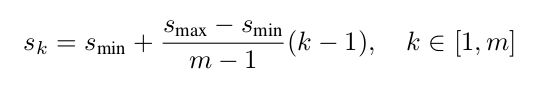
论文给定Smin=0.2,Smax=0.9,然后根据上面公式计算k表示第一个特征图,计算得到每层的sk,然后计算长和宽,计算公式如下:

当长宽比为1的时候,

多加一个上面的,但是代码不是这样实现的,他是直接给了长宽,我们看看,
 anchor_sizes=[(20.48, 51.2),
                      (51.2, 133.12),
                      (133.12, 215.04),
                      (215.04, 296.96),
                      (296.96, 378.88),
                      (378.88, 460.8),
                      (460.8, 542.72)],
        anchor_ratios=[[2, .5],
                       [2, .5, 3, 1./3],
                       [2, .5, 3, 1./3],
                       [2, .5, 3, 1./3],
                       [2, .5, 3, 1./3],
                       [2, .5],
                       [2, .5]],
我们看到他的Sk是大小,不是比例,论文上是0.2-0.9,而且你用512×0.2计算得到的也不是代码给的,所以这个地方其实框的大小是可以自己给的,可以根据经验给定。根据上面的计算得到框的大小。
最后是返回一个改层每个中心点坐标和框。存在layers_anchors,并返回,这个地方其实和Faster-Rcnn是一样的。也是anchor机制。
3 对anchor和GT的预处理
我们看代码:
    def bboxes_encode(self, labels, bboxes, anchors,
                      scope=None):
        """Encode labels and bounding boxes.
        """
        return ssd_common.tf_ssd_bboxes_encode(
            labels, bboxes, anchors,
            self.params.num_classes,
            self.params.no_annotation_label,
            ignore_threshold=0.5,
            prior_scaling=self.params.prior_scaling,
            scope=scope)
一看就知道是调用了ssd_common.tf_ssd_bboxes_encode这个函数,我们看看:
def tf_ssd_bboxes_encode(labels,
                         bboxes,
                         anchors,
                         num_classes,
                         no_annotation_label,
                         ignore_threshold=0.5,
                         prior_scaling=[0.1, 0.1, 0.2, 0.2],
                         dtype=tf.float32,
                         scope='ssd_bboxes_encode'):
    """Encode groundtruth labels and bounding boxes using SSD net anchors.
    Encoding boxes for all feature layers.

    Arguments:
      labels: 1D Tensor(int64) containing groundtruth labels;
      bboxes: Nx4 Tensor(float) with bboxes relative coordinates;
      anchors: List of Numpy array with layer anchors;
      matching_threshold: Threshold for positive match with groundtruth bboxes;
      prior_scaling: Scaling of encoded coordinates.

    Return:
      (target_labels, target_localizations, target_scores):
        Each element is a list of target Tensors.
    """
    with tf.name_scope(scope):
        target_labels = []
        target_localizations = []
        target_scores = []
        for i, anchors_layer in enumerate(anchors):
            with tf.name_scope('bboxes_encode_block_%i' % i):
                t_labels, t_loc, t_scores = \
                    tf_ssd_bboxes_encode_layer(labels, bboxes, anchors_layer,
                                               num_classes, no_annotation_label,
                                               ignore_threshold,
                                               prior_scaling, dtype)
                target_labels.append(t_labels)
                target_localizations.append(t_loc)
                target_scores.append(t_scores)
        ## t_labels 表示返回每个anchor对应的类别,t_loc返回的是一种变换,
        ## t_scores 每个anchor与gt对应的最大的交并比
        ## target_labels是一个list,包含每层的每个anchor对应的gt类别,
        ## target_localizations对应的是包含每一层所有anchor对应的变换
        ### target_scores 返回的是每个anchor与gt对应的最大的交并比
        return target_labels, target_localizations, target_scores
看上面的函数就知道,他们有是调用了tf.ssd_bboxes_encode_layer这个函数,有一个循环,是对需要预测的特征图一层一层的循环,然后我们看调用的函数
def tf_ssd_bboxes_encode_layer(labels,
                               bboxes,
                               anchors_layer,
                               num_classes,
                               no_annotation_label,
                               ignore_threshold=0.5,
                               prior_scaling=[0.1, 0.1, 0.2, 0.2],
                               dtype=tf.float32):
    """Encode groundtruth labels and bounding boxes using SSD anchors from
    one layer.

    Arguments:
      labels: 1D Tensor(int64) containing groundtruth labels;
      bboxes: Nx4 Tensor(float) with bboxes relative coordinates;
      anchors_layer: Numpy array with layer anchors;
      matching_threshold: Threshold for positive match with groundtruth bboxes;
      prior_scaling: Scaling of encoded coordinates.

    Return:
      (target_labels, target_localizations, target_scores): Target Tensors.
    """
    # Anchors coordinates and volume.
    yref, xref, href, wref = anchors_layer
    ymin = yref - href / 2.
    xmin = xref - wref / 2.
    ymax = yref + href / 2.
    xmax = xref + wref / 2.
    vol_anchors = (xmax - xmin) * (ymax - ymin)

    # Initialize tensors...
    shape = (yref.shape[0], yref.shape[1], href.size)
    feat_labels = tf.zeros(shape, dtype=tf.int64)
    feat_scores = tf.zeros(shape, dtype=dtype)

    feat_ymin = tf.zeros(shape, dtype=dtype)
    feat_xmin = tf.zeros(shape, dtype=dtype)
    feat_ymax = tf.ones(shape, dtype=dtype)
    feat_xmax = tf.ones(shape, dtype=dtype)

    def jaccard_with_anchors(bbox):
        """Compute jaccard score between a box and the anchors.
        """
        int_ymin = tf.maximum(ymin, bbox[0])
        int_xmin = tf.maximum(xmin, bbox[1])
        int_ymax = tf.minimum(ymax, bbox[2])
        int_xmax = tf.minimum(xmax, bbox[3])
        h = tf.maximum(int_ymax - int_ymin, 0.)
        w = tf.maximum(int_xmax - int_xmin, 0.)
        # Volumes.
        inter_vol = h * w
        union_vol = vol_anchors - inter_vol \
            + (bbox[2] - bbox[0]) * (bbox[3] - bbox[1])
        jaccard = tf.div(inter_vol, union_vol)
        return jaccard

    def intersection_with_anchors(bbox):
        """Compute intersection between score a box and the anchors.
        """
        int_ymin = tf.maximum(ymin, bbox[0])
        int_xmin = tf.maximum(xmin, bbox[1])
        int_ymax = tf.minimum(ymax, bbox[2])
        int_xmax = tf.minimum(xmax, bbox[3])
        h = tf.maximum(int_ymax - int_ymin, 0.)
        w = tf.maximum(int_xmax - int_xmin, 0.)
        inter_vol = h * w
        scores = tf.div(inter_vol, vol_anchors)
        return scores

    def condition(i, feat_labels, feat_scores,
                  feat_ymin, feat_xmin, feat_ymax, feat_xmax):
        """Condition: check label index.
        """
        ### 逐元素比较大小,其实就是遍历label,因为i在body返回的时候加1了,直到遍历完
        r = tf.less(i, tf.shape(labels))
        return r[0]

    def body(i, feat_labels, feat_scores,
             feat_ymin, feat_xmin, feat_ymax, feat_xmax):
        """Body: update feature labels, scores and bboxes.
        Follow the original SSD paper for that purpose:
          - assign values when jaccard > 0.5;
          - only update if beat the score of other bboxes.
        """
        # Jaccard score.
        label = labels[i]
        bbox = bboxes[i]
        ### 返回的是交并比,算某一层上所有的框和图像中第一个框的交并比
        jaccard = jaccard_with_anchors(bbox)
        # Mask: check threshold + scores + no annotations + num_classes.
        ### 这个地方是帅选掉交并比小于0的
        mask = tf.greater(jaccard, feat_scores)
        # mask = tf.logical_and(mask, tf.greater(jaccard, matching_threshold))

        mask = tf.logical_and(mask, feat_scores > -0.5)
        mask = tf.logical_and(mask, label < num_classes)
        imask = tf.cast(mask, tf.int64)
        fmask = tf.cast(mask, dtype)
        # Update values using mask.
        feat_labels = imask * label + (1 - imask) * feat_labels
        ## tf.where表示如果mask为镇则jaccard,否则为feat_scores
        feat_scores = tf.where(mask, jaccard, feat_scores)
        ###
        feat_ymin = fmask * bbox[0] + (1 - fmask) * feat_ymin
        feat_xmin = fmask * bbox[1] + (1 - fmask) * feat_xmin
        feat_ymax = fmask * bbox[2] + (1 - fmask) * feat_ymax
        feat_xmax = fmask * bbox[3] + (1 - fmask) * feat_xmax

        # Check no annotation label: ignore these anchors...
        # interscts = intersection_with_anchors(bbox)
        # mask = tf.logical_and(interscts > ignore_threshold,
        #                       label == no_annotation_label)
        # # Replace scores by -1.
        # feat_scores = tf.where(mask, -tf.cast(mask, dtype), feat_scores)

        return [i+1, feat_labels, feat_scores,
                feat_ymin, feat_xmin, feat_ymax, feat_xmax]
    # Main loop definition.
    i = 0
    [i, feat_labels, feat_scores,
     feat_ymin, feat_xmin,
     feat_ymax, feat_xmax] = tf.while_loop(condition, body,
                                           [i, feat_labels, feat_scores,
                                            feat_ymin, feat_xmin,
                                            feat_ymax, feat_xmax])
    # Transform to center / size.
    feat_cy = (feat_ymax + feat_ymin) / 2.
    feat_cx = (feat_xmax + feat_xmin) / 2.
    feat_h = feat_ymax - feat_ymin
    feat_w = feat_xmax - feat_xmin
    # Encode features.
    ### prior_scaling=[0.1, 0.1, 0.2, 0.2]
    feat_cy = (feat_cy - yref) / href / prior_scaling[0]
    feat_cx = (feat_cx - xref) / wref / prior_scaling[1]
    feat_h = tf.log(feat_h / href) / prior_scaling[2]
    feat_w = tf.log(feat_w / wref) / prior_scaling[3]
    # Use SSD ordering: x / y / w / h instead of ours.
    feat_localizations = tf.stack([feat_cx, feat_cy, feat_w, feat_h], axis=-1)
    ## feat_labels 表示返回每个anchor对应的类别,feat_localizations返回的是一种变换,
    ## feat_scores 每个anchor与gt对应的最大的交并比
    return feat_labels, feat_localizations, feat_scores
看这部分写的有点不太好读,因为他是函数里面写函数,调用自己的函数,关键是他把自己写的函数放在中间,使得代码前面一半后面一半,中间是一些函数,不仔细往后看还以为结束了。
yref, xref, href, wref = anchors_layer
ymin = yref - href / 2.
xmin = xref - wref / 2.
ymax = yref + href / 2.
xmax = xref + wref / 2.
vol_anchors = (xmax - xmin) * (ymax - ymin)

# Initialize tensors...
shape = (yref.shape[0], yref.shape[1], href.size)
feat_labels = tf.zeros(shape, dtype=tf.int64)
feat_scores = tf.zeros(shape, dtype=dtype)

feat_ymin = tf.zeros(shape, dtype=dtype)
feat_xmin = tf.zeros(shape, dtype=dtype)
feat_ymax = tf.ones(shape, dtype=dtype)
feat_xmax = tf.ones(shape, dtype=dtype)
开头是这样的,ymin,xmin,ymax,xmax之类的是把之前的坐标换成了左上角和右上角的坐标,方便求交并比,注意这个地方像y_ref之类的都是一个numpy数组,是整个特征图所以的中心点,所以这个地方相当于是numpy的广播性质,可不是一个框的操作,而是整个层的操作,shape是tensor的形状,feat_labels,feat_scores,feat_ymin这些是为了保存结果的,形状应该和我们框坐标之类的一样。
接下来,应该跳过那些函数,看后面的
# Main loop definition.
i = 0
[i, feat_labels, feat_scores,
 feat_ymin, feat_xmin,
 feat_ymax, feat_xmax] = tf.while_loop(condition, body,
                                       [i, feat_labels, feat_scores,
                                        feat_ymin, feat_xmin,
                                        feat_ymax, feat_xmax])
# Transform to center / size.
feat_cy = (feat_ymax + feat_ymin) / 2.
feat_cx = (feat_xmax + feat_xmin) / 2.
feat_h = feat_ymax - feat_ymin
feat_w = feat_xmax - feat_xmin
# Encode features.
### prior_scaling=[0.1, 0.1, 0.2, 0.2]
feat_cy = (feat_cy - yref) / href / prior_scaling[0]
feat_cx = (feat_cx - xref) / wref / prior_scaling[1]
feat_h = tf.log(feat_h / href) / prior_scaling[2]
feat_w = tf.log(feat_w / wref) / prior_scaling[3]
# Use SSD ordering: x / y / w / h instead of ours.
feat_localizations = tf.stack([feat_cx, feat_cy, feat_w, feat_h], axis=-1)
tf.while_loop()这个函数是如果满足condition,则执行body,当然传递的参数就是后面的list,那我们看condition函数,
def condition(i, feat_labels, feat_scores,
              feat_ymin, feat_xmin, feat_ymax, feat_xmax):

    ### 逐元素比较大小,其实就是遍历label,因为i在body返回的时候加1了,直到遍历完
    r = tf.less(i, tf.shape(labels))
    return r[0]
我上面解释的很清楚,tf.less表示逐元素比较大小,就是如果i
def body(i, feat_labels, feat_scores,
         feat_ymin, feat_xmin, feat_ymax, feat_xmax):

    label = labels[i]
    bbox = bboxes[i]
    ### 返回的是交并比,算某一层上所有的框和图像中第一个框的交并比
    jaccard = jaccard_with_anchors(bbox)
    # Mask: check threshold + scores + no annotations + num_classes.
    ### 这个地方是帅选掉交并比小于0的
    mask = tf.greater(jaccard, feat_scores)
    # mask = tf.logical_and(mask, tf.greater(jaccard, matching_threshold))
    mask = tf.logical_and(mask, feat_scores > -0.5)
    mask = tf.logical_and(mask, label < num_classes)
    imask = tf.cast(mask, tf.int64)
    fmask = tf.cast(mask, dtype)
    # Update values using mask.
    feat_labels = imask * label + (1 - imask) * feat_labels
    ## tf.where表示如果mask为镇则jaccard,否则为feat_scores
    feat_scores = tf.where(mask, jaccard, feat_scores)

    feat_ymin = fmask * bbox[0] + (1 - fmask) * feat_ymin
    feat_xmin = fmask * bbox[1] + (1 - fmask) * feat_xmin
    feat_ymax = fmask * bbox[2] + (1 - fmask) * feat_ymax
    feat_xmax = fmask * bbox[3] + (1 - fmask) * feat_xmax


    return [i+1, feat_labels, feat_scores,
            feat_ymin, feat_xmin, feat_ymax, feat_xmax]
jaccard_with_anchors 这个函数其实就是返回交并比,
def jaccard_with_anchors(bbox):
    """Compute jaccard score between a box and the anchors.
    """
    int_ymin = tf.maximum(ymin, bbox[0])
    int_xmin = tf.maximum(xmin, bbox[1])
    int_ymax = tf.minimum(ymax, bbox[2])
    int_xmax = tf.minimum(xmax, bbox[3])
    h = tf.maximum(int_ymax - int_ymin, 0.)
    w = tf.maximum(int_xmax - int_xmin, 0.)
    # Volumes.
    inter_vol = h * w
    union_vol = vol_anchors - inter_vol \
        + (bbox[2] - bbox[0]) * (bbox[3] - bbox[1])
    jaccard = tf.div(inter_vol, union_vol)
    return jaccard
先求相交的坐标,然后求相交的面积,然后求交并比,比较简单。
这个地方是帅选掉交并比小于0的
mask = tf.greater(jaccard, feat_scores)
tf.greater就是比较大小,如果jaccard>feat_scores则为真,否则为假。tf.logical_and表示两个同时为真才是真,
feat_labels = imask * label + (1 - imask) * feat_labels
上面这一句,当imask为1,那么就是label,否则label就是0,也就是背景,那imask什么时候为1,imask = tf.cast(mask, tf.int64),而mask又是大于feat_score的,所以这个地方因为是循环,遍历所有的目标,那么选择框的方式就是,选择交比比最大的,也就是某一个目标他对应的框里面,交并比最大的,这是一种策略,但是论文中还提到,高于0.5的我们也有对应的目标,但是代码没有这中策略,它只是选择了交并比最大的。feat_scores = tf.where(mask, jaccard, feat_scores),这个地方就是更新feat_scores,也就是体现是选择交并比最大的。
后面的feat_ymin之类的,也是跟着更新,如果该框的交并比大,那么就是保存为GT的bbox,然后返回,进行下一个循环。循环完了我们看后面的代码:
# Transform to center / size.
feat_cy = (feat_ymax + feat_ymin) / 2.
feat_cx = (feat_xmax + feat_xmin) / 2.
feat_h = feat_ymax - feat_ymin
feat_w = feat_xmax - feat_xmin
# Encode features.
### prior_scaling=[0.1, 0.1, 0.2, 0.2]
feat_cy = (feat_cy - yref) / href / prior_scaling[0]
feat_cx = (feat_cx - xref) / wref / prior_scaling[1]
feat_h = tf.log(feat_h / href) / prior_scaling[2]
feat_w = tf.log(feat_w / wref) / prior_scaling[3]
# Use SSD ordering: x / y / w / h instead of ours.
feat_localizations = tf.stack([feat_cx, feat_cy, feat_w, feat_h], axis=-1)
## feat_labels 表示返回每个anchor对应的类别,feat_localizations返回的是一种变换,
## feat_scores 每个anchor与gt对应的最大的交并比
return feat_labels, feat_localizations, feat_scores
feat_cy之类的是框的左上角和右下角坐标变为中心左边和场合宽,还是一样的,是numpy的广播,这个特征层一起变,
prior_scaling这个其实我也不知道到为啥需要缩放,貌似论文没说要缩放,终点看这一快
feat_cy = (feat_cy - yref) / href / prior_scaling[0]
feat_cx = (feat_cx - xref) / wref / prior_scaling[1]
feat_h = tf.log(feat_h / href) / prior_scaling[2]
feat_w = tf.log(feat_w / wref) / prior_scaling[3]
这个其实就是论文的这个一块,

其实和我们的Faster rcnn是一样的,是求真实框与anchor之间的变换,你把上面随便一个移项,就会得anchor经过伸缩变换得到真实的框,所以这个地方回归的是一种变换,因为实际我们的框是存在的,然后经过我们回归得到的变换,经过变换得到真实框,所以这个地方损失函数其实是我们预测的是变换,我们实际的框和anchor之间的变换和我们预测的变换之间的loss。我们回归的是一种变换。并不是直接预测框,这个和YOLO是不一样的。和Faster RCNN是一样的。然后返回每一层的结果,放在
target_labels.append(t_labels)
target_localizations.append(t_loc)
target_scores.append(t_scores)
## t_labels 表示返回每个anchor对应的类别,t_loc返回的是一种变换,
## t_scores 每个anchor与gt对应的最大的交并比
## target_labels是一个list,包含每层的每个anchor对应的gt类别,
## target_localizations对应的是包含每一层所有anchor对应的变换
### target_scores 返回的是每个anchor与gt对应的最大的交并比
接下来我们看损失函数:
4 SSD 损失函数
我们先看代码:
    def losses(self, logits, localisations,
               gclasses, glocalisations, gscores,
               match_threshold=0.5,
               negative_ratio=3.,
               alpha=1.,
               label_smoothing=0.,
               scope='ssd_losses'):
        """Define the SSD network losses.
        """
        return ssd_losses(logits, localisations,
                          gclasses, glocalisations, gscores,
                          match_threshold=match_threshold,
                          negative_ratio=negative_ratio,
                          alpha=alpha,
                          label_smoothing=label_smoothing,
                          scope=scope)
这个地方也是调用其他函数,所以这个代码读起来挺费劲的,都是这个调那个,解释以下参数的含义,logits是每一层特征图输出,是没有经过softmax的,localistions是我们的预测框,带g的表示真实的,negative是正反例之比,是1:3,也就是负例是3,这个地方和论文是一样的。label_smoothing这个地方设置为0,并没有做平滑,记得在GAN的loss里面会用到。
然后我们看ssd_losses这个函数:
def ssd_losses(logits, localisations,
               gclasses, glocalisations, gscores,
               match_threshold=0.5,
               negative_ratio=3.,
               alpha=1.,
               label_smoothing=0.,
               scope=None):
    """Loss functions for training the SSD 300 VGG network.

    This function defines the different loss components of the SSD, and
    adds them to the TF loss collection.

    Arguments:
      logits: (list of) predictions logits Tensors;
      localisations: (list of) localisations Tensors;
      gclasses: (list of) groundtruth labels Tensors;
      glocalisations: (list of) groundtruth localisations Tensors;
      gscores: (list of) groundtruth score Tensors;
    """
    with tf.name_scope(scope, 'ssd_losses'):
        l_cross_pos = []
        l_cross_neg = []
        l_loc = []
        for i in range(len(logits)):
            dtype = logits[i].dtype
            with tf.name_scope('block_%i' % i):
                # Determine weights Tensor.
                pmask = gscores[i] > match_threshold
                fpmask = tf.cast(pmask, dtype)
                n_positives = tf.reduce_sum(fpmask)

                # Select some random negative entries.
                # n_entries = np.prod(gclasses[i].get_shape().as_list())
                # r_positive = n_positives / n_entries
                # r_negative = negative_ratio * n_positives / (n_entries - n_positives)

                # Negative mask.
                no_classes = tf.cast(pmask, tf.int32)
                predictions = slim.softmax(logits[i])
                nmask = tf.logical_and(tf.logical_not(pmask),
                                       gscores[i] > -0.5)
                fnmask = tf.cast(nmask, dtype)
                nvalues = tf.where(nmask,
                                   predictions[:, :, :, :, 0],
                                   1. - fnmask)
                nvalues_flat = tf.reshape(nvalues, [-1])
                # Number of negative entries to select.
                n_neg = tf.cast(negative_ratio * n_positives, tf.int32)
                n_neg = tf.maximum(n_neg, tf.size(nvalues_flat) // 8)
                n_neg = tf.maximum(n_neg, tf.shape(nvalues)[0] * 4)
                max_neg_entries = 1 + tf.cast(tf.reduce_sum(fnmask), tf.int32)
                n_neg = tf.minimum(n_neg, max_neg_entries)

                val, idxes = tf.nn.top_k(-nvalues_flat, k=n_neg)
                minval = val[-1]
                # Final negative mask.
                nmask = tf.logical_and(nmask, -nvalues > minval)
                fnmask = tf.cast(nmask, dtype)

                # Add cross-entropy loss.
                with tf.name_scope('cross_entropy_pos'):
                    loss = tf.nn.sparse_softmax_cross_entropy_with_logits(logits=logits[i],
                                                                          labels=gclasses[i])
                    loss = tf.losses.compute_weighted_loss(loss, fpmask)
                    l_cross_pos.append(loss)

                with tf.name_scope('cross_entropy_neg'):
                    loss = tf.nn.sparse_softmax_cross_entropy_with_logits(logits=logits[i],
                                                                          labels=no_classes)
                    loss = tf.losses.compute_weighted_loss(loss, fnmask)
                    l_cross_neg.append(loss)

                # Add localization loss: smooth L1, L2, ...
                with tf.name_scope('localization'):
                    # Weights Tensor: positive mask + random negative.
                    weights = tf.expand_dims(alpha * fpmask, axis=-1)
                    loss = custom_layers.abs_smooth(localisations[i] - glocalisations[i])
                    loss = tf.losses.compute_weighted_loss(loss, weights)
                    l_loc.append(loss)

        # Additional total losses...
        with tf.name_scope('total'):
            total_cross_pos = tf.add_n(l_cross_pos, 'cross_entropy_pos')
            total_cross_neg = tf.add_n(l_cross_neg, 'cross_entropy_neg')
            total_cross = tf.add(total_cross_pos, total_cross_neg, 'cross_entropy')
            total_loc = tf.add_n(l_loc, 'localization')

            # Add to EXTRA LOSSES TF.collection
            tf.add_to_collection('EXTRA_LOSSES', total_cross_pos)
            tf.add_to_collection('EXTRA_LOSSES', total_cross_neg)
            tf.add_to_collection('EXTRA_LOSSES', total_cross)
tf.add_to_collection('EXTRA_LOSSES', total_loc)pmask = gscores[i] > match_threshold fpmask = tf.cast(pmask, dtype) n_positives = tf.reduce_sum(fpmask)
这个代码,这个地方又做一次帅选,如果交并比大于0.5,那么我们认为是正例,fpmask 记录正例和负例,n_positives这个是
正例的个数,
no_classes = tf.cast(pmask, tf.int32)
predictions = slim.softmax(logits[i])
nmask = tf.logical_and(tf.logical_not(pmask),
                       gscores[i] > -0.5)
fnmask = tf.cast(nmask, dtype)
nvalues = tf.where(nmask,
                   predictions[:, :, :, :, 0],
                   1. - fnmask)
nvalues_flat = tf.reshape(nvalues, [-1])
no_classes把布尔型变量变为整形,那么就是要么是0,要么是1,前景就是1,背景就是0,predictions是记录预测每个类的概率
nmask,就是负例,你看,tf.logical_not(pmask)就是取反,这个地方我觉得gscores[i] > -0.5,之前已经帅选了,就
是交并比不合适的,小于0的,这个地方应该。
nvalues就是把我们的类别提取出来,否则就是0,表示背景。后面就是做了一个拉伸。tf.where(cond,x,y)表示如果cond为真,就是x,否则就是y。
n_neg = tf.cast(negative_ratio * n_positives, tf.int32)
n_neg = tf.maximum(n_neg, tf.size(nvalues_flat) // 8)
n_neg = tf.maximum(n_neg, tf.shape(nvalues)[0] * 4)
max_neg_entries = 1 + tf.cast(tf.reduce_sum(fnmask), tf.int32)
n_neg = tf.minimum(n_neg, max_neg_entries)

val, idxes = tf.nn.top_k(-nvalues_flat, k=n_neg)
minval = val[-1]
# Final negative mask.
nmask = tf.logical_and(nmask, -nvalues > minval)
fnmask = tf.cast(nmask, dtype)
n_neg就是负样本的数量, negative_ratio正负样本比列,默认就是3,后面的第一个取最大,我觉得是保证至少有负样本,
max_neg_entries这个就是负样本的数量,n_neg = tf.minimum(n_neg, max_neg_entries),这个比较很好理解,万一
你总样本比你三倍正样本少,所以需要选择小的,所以这个地方保证足够的负样本,nmask表示我们所选取的负样本,
tf.nn.top_k,这个是选取前k=neg个负例,因为取了负号,表示选择的交并比最小的k个,minval就是选择负例里面交并比
最大的,nmask就是把我们选择的负样例设为整数,就是提取出我们选择的,tf.logical_and就是同时为真,首先。需要是
负例,其次值需要大于minval,因为取了负数,所以nmask就是我们所选择的负例,fnmask就是就是我们选取的负样本只是
数据类型变了,由bool变为了浮点型,(dtype默认是浮点型),接着看损失函数:
# Add cross-entropy loss.
with tf.name_scope('cross_entropy_pos'):
    loss = tf.nn.sparse_softmax_cross_entropy_with_logits(logits=logits[i],
                                                          labels=gclasses[i])
    loss = tf.losses.compute_weighted_loss(loss, fpmask)
    l_cross_pos.append(loss)
这个是正例的损失,其实就是交叉熵损失,tf.losses.compute_weighted_loss其实就是相当于loss×fpmask,
这个地方之所以需要乘以fpmask是为了过滤掉负样本,因为负样本的label就是0,其他得是1.而fpmask刚好就是这样。
with tf.name_scope('cross_entropy_neg'):
    loss = tf.nn.sparse_softmax_cross_entropy_with_logits(logits=logits[i],
                                                          labels=no_classes)
    loss = tf.losses.compute_weighted_loss(loss, fnmask)
    l_cross_neg.append(loss)
这个是负例的损失函数,也是交叉熵损失,同时fnmask也是过滤掉正例,no_classes里面负例就是0,
                with tf.name_scope('localization'):
                    # Weights Tensor: positive mask + random negative.
                    weights = tf.expand_dims(alpha * fpmask, axis=-1)
                    loss = custom_layers.abs_smooth(localisations[i] - glocalisations[i])
                    loss = tf.losses.compute_weighted_loss(loss, weights)
                    l_loc.append(loss)
这个地方就是回归框损失,我们先看看论文回归框损失用的损失函数,就是smoothL1损失,这个样子:

然后我们再看这个函数代码:
def abs_smooth(x):
    """Smoothed absolute function. Useful to compute an L1 smooth error.

    Define as:
        x^2 / 2         if abs(x) < 1
        abs(x) - 0.5    if abs(x) > 1
    We use here a differentiable definition using min(x) and abs(x). Clearly
    not optimal, but good enough for our purpose!
    """
    absx = tf.abs(x)
    minx = tf.minimum(absx, 1)
    r = 0.5 * ((absx - 1) * minx + absx)
    return r
其实就是上面的损失函数,然后后面的weight也是过滤框没有目标的,之所有alpha是因为论文也有,但是默认就是1,现在我们看看论文的损失函数
其实和论文的损失函数是一样的。
关于代码,代码的训练部分还有很多其他内容,涉及多gpu,预处理等,但是核心思想就是这些,有机会在将其他的代码。