透彻理解线性回归 (公式推导+python实现+应用举例+sklearn应用)

线性回归 (公式推导+python实现+应用举例+sklearn应用)

1.公式推导

---

线性模型形式如下:

hθ(x)=θ0x0+θ1x1+⋯+θnxn=∑i=1nθixi h θ ( x ) = θ 0 x 0 + θ 1 x 1 + ⋯ + θ n x n = ∑ i = 1 n θ i x i

写成向量形式即:

hθ(x)=θTx+b h θ ( x ) = θ T x + b

而我们的损失函数为:

J(θ)=12m(hθ(x(i))−y(i))2=12m∑i=1n(hθ(x(i))−y(i))2 J ( θ ) = 1 2 m ( h θ ( x ( i ) ) − y ( i ) ) 2 = 1 2 m ∑ i = 1 n ( h θ ( x ( i ) ) − y ( i ) ) 2

推广到有m个样本的情形，将其转化为矩阵表达形式，即:

hθ(X)=Xθ h θ ( X ) = X θ

把 均方误差(mean square error)即 欧氏距离(Euclidean distance)除以2m得到我们的 损失函数(cost functino): 注: 基于均方误差最小化来进行模型求解的方法叫做最小二乘法(least square method)

J(θ)=12m(Xθ−Y)T(Xθ−Y)=12m(θTXT−YT)(Xθ−Y)=12m(θTXTXθ−θTXTY−YTXθ+YTY)(16)(17)(18) (16) J ( θ ) = 1 2 m ( X θ − Y ) T ( X θ − Y ) (17) = 1 2 m ( θ T X T − Y T ) ( X θ − Y ) (18) = 1 2 m ( θ T X T X θ − θ T X T Y − Y T X θ + Y T Y )

补充下矩阵求导法则:

dABdB=AT d A B d B = A T

dATBdA=B d A T B d A = B

dXTAXdX=2AX d X T A X d X = 2 A X

设我们有m个样本，n个属性，则X是m * (n+1) 矩阵(第1列全为1), 而 θ θ 是n+1维向量, 对 J(θ) J ( θ ) 求导:

∂J(θ)∂θ=12m(2XTXθ−XTY−XTY)=1mXT(Xθ−Y)(19)(20) (19) ∂ J ( θ ) ∂ θ = 1 2 m ( 2 X T X θ − X T Y − X T Y ) (20) = 1 m X T ( X θ − Y )

要求最小值，先令其为0,得到:

θ=(XTX)−1XTY θ = ( X T X ) − 1 X T Y

将 θ θ 代入线性模型得到:

hθ(X)=X(XTX)−1XTY h θ ( X ) = X ( X T X ) − 1 X T Y

这是我们直接得出的结果，但是有两点需要注意:
1. 这是建立在 XTX X T X 可逆的基础上，若其不可逆则不能用该公式
2. 计算量实在是太大了,光是 (XTX)−1 ( X T X ) − 1 就需要计算(n+1) * (n+1)矩阵的逆

综上，实际中往往采用的是梯度下降(Gradient Descent)方法:

因为代价函数对 θj θ j 求偏导得到:

∂J(θ)∂θj=1m∑i=1n(hθ(xi)−yi)xj ∂ J ( θ ) ∂ θ j = 1 m ∑ i = 1 n ( h θ ( x i ) − y i ) x j

则对 θ θ 的更新如下:
- until convergence:{
   for j in 1…n+1{

θj:=θj−α1m∑i=1n(hθ(xi)−yi)xj θ j := θ j − α 1 m ∑ i = 1 n ( h θ ( x i ) − y i ) x j

   }
}

同样地，将其转化为矩阵形式
注:这里 α α 是学习速率, θ θ 是(n+1, 1)的向量; X是(m, n+1)的矩阵; Y是(m, 1)的向量, hθ(X) h θ ( X ) 也是(m, 1)的向量:

θ=θ−αmXT⋅(hθ(X)−Y) θ = θ − α m X T ⋅ ( h θ ( X ) − Y )

注意 θ θ 是一个数，所以这里用的是点乘

---

2.用数据举例

这里导入的是高炉数据，高炉的含硅(Si)量预测可是个经典的问题
首先获取原始数据的DataFrame : data

import numpy as np
import matplotlib.pyplot as plt
import pandas as pd
# 这是我的环境需要，大多数人并不需要加以下两行代码
import sys
sys.path.append("C:\\python\\lib\\site-packages")
%matplotlib inline

data = pd.read_csv("raw/blast _furnance.csv")
print(data.describe())

得到结果:

	Si	S	coal	wind
count	1000.000000	1000.000000	1000.000000	1000.000000
mean	0.459410	0.023788	13.159400	1759.686810
std	0.110965	0.009743	2.121651	80.083738
min	0.210000	0.006000	0.120000	833.520000
25%	0.380000	0.017000	12.447500	1733.732500
50%	0.440000	0.023000	13.545000	1775.240000
75%	0.520000	0.030000	14.370000	1802.390000
max	1.260000	0.078000	17.700000	1897.230000

可以看到，该数据集分为3个特征: S(含硫量), coal(喷煤量), wind(风量)
且一共有1000条数据，不存在数据缺失

---

* 简单介绍下归一化和标准化

现在我们需要对数据预处理，即归一化(Normalization) 或 标准化(Standardization)

• 什么是归一化 (归一化目标是啥)
  1.把数据映射到(0, 1)之间
  2.去量纲化
• 和标准化的区别是啥
  标准化不会改变数据的分布,归一化会改变数据分布

• 为什么要做归一化
  1.提升模型的收敛(convergence)速度
  如果没有做归一化，各特征尺度不一样的话，会造成目标函数整个图形特别狭长，梯度下降的过程会走很多”弯路”
  2.有助于提升模型的精度
  这在牵涉到距离计算的算法如SVM时，提升效果非常显著, 因为如果这个特征变化特别大，距离计算就主要取决于这个特征，不符合实际情况

• 常用归一化算法:
  线性转换:

  y=x−minmax−min y = x − min max − min

• 常用标准化算法:
  1.MinMax规范化(线性变换):
  y=x−minmax−min∗(max^−min^)+min^ y = x − min max − min ∗ ( max ^ − min ^ ) + min ^
  
  注: max^、min^ m a x ^ 、 m i n ^ 分别是新的最大值与最小值
  
  2.Z-Score规范化(标准差标准化):
  y=x−X¯maxX−minX=x−μσ y = x − X ¯ max X − min X = x − μ σ
  
  注: 经过处理的数据符合标准正态分布，均值为0，标准差为1
  
  3.对数Logistic规范化 :
  y=11+e−x y = 1 1 + e − x
  
  4.log函数规范化 :
  x=lgxlgmax(x) x = lg ⁡ x lg ⁡ m a x ( x )
  
  注: 属于非线性的标准化，适用于数据分化大的场景，有些值特别大，有些值特别小
  

这里我们选择手动实现一个Z-Score的标准化:

def standard(X):
    # np.array() 可将其它一些数据转化为numpy.ndarray类型的数据方便进行矩阵运算, 而np.ndarray()是将其它numpy.ndarray作为输入
    X_norm = np.array(X)

    # 创建一个1行，和X列宽等长的行向量
    mu = np.zeros((1, X.shape[1]))
    sigma = np.zeros((1, X.shape[1]))

    mu = np.mean(X_norm, axis=0) # 求每一列的平均值，axis=0指定求的是列的均值
    sigma = np.std(X_norm, axis=0)
    for i in range(X.shape[1]): # 遍历每一列
        X_norm[: ,i] = (X_norm[: ,i] - mu[i]) / sigma[i]

    return X_norm, mu, sigma

data_norm, mu, sigma = standard(data)
print(data_norm)

得到结果:

array([[ 0.18564659, -0.38900304, -0.48071521, -1.441423  ],
       [ 0.36597354, -1.41593821, -0.72592996, -1.33435646],
       [-0.35533425, -1.41593821, -1.33896682, -0.70095235],
       ..., 
       [-0.1750073 , -1.21055117, -0.45242121, -1.71614797],
       [ 0.00531965,  0.22715806, -0.99943871, -0.60125679],
       [-0.71598815, -0.90247062,  0.4954281 , -1.00253766]])

接下来我们data_norm再分割为Samples(样本矩阵)和Labels(结果向量)

Samples = data_norm[:, 1:]
print(Samples)

结果如下

array([[-0.38900304, -0.48071521, -1.441423  ],
       [-1.41593821, -0.72592996, -1.33435646],
       [-1.41593821, -1.33896682, -0.70095235],
       ..., 
       [-1.21055117, -0.45242121, -1.71614797],
       [ 0.22715806, -0.99943871, -0.60125679],
       [-0.90247062,  0.4954281 , -1.00253766]])

再检查标记向量:

Labels = data_norm[:, 0:1]
print(Labels.shape)

结果如下:

(1000, 1)

3.python实现线性回归

"""
    代价函数
    X是样本矩阵(m, n+1), y是结果向量(m, 1), theta是参数向量(n+1, 1)
    返回一个数，即代价值
"""
def get_cost(X, y, theta):
    # 对numpy.ndarray来说，np.dot()才是真正的线性代数中的矩阵相乘
    return np.dot((np.transpose(np.dot(X,theta) - y)) , (np.dot(X,theta) - y)) / (2*y.shape[0])

"""
    计算梯度下降, 返回最终学得的theta向量和cost function的变化list
    X: (m, n+1)样本矩阵
    y: (m, 1)结果向量
    theta: (n+1, 1)参数向量
    rate: 学习速率
    rounds: 训练轮次
    intercept: 若为True,则需要给样本矩阵X增加常数列
"""
def gradient_descent(X, y, rate, rounds, intercept=True):
    iX = X.copy() # 如果不用copy()函数，改变iX同样会改变X
    if intercept == True:
        iX = np.column_stack((np.ones(iX.shape[0]), iX)) # 给第一列全加上1

    T = np.full(shape=(iX.shape[1], 1), fill_value=0.5, dtype=np.float)
    L, costs = [], []

    for i in range(rounds):
        H = np.dot(iX, T) # 求内积，先计算出假设函数
        T = T - (rate/y.shape[0]) * np.dot(np.transpose(iX), (H-y))
        L.append(i)
        costs.append(get_cost(iX, y, T).tolist()[0])

    return T, costs

训练一个模型出来:

Theta, Costs = gradient_descent(Samples, Labels, 0.1, 40)

再绘出训练过程中代价函数变化曲线:

plt.plot(Costs)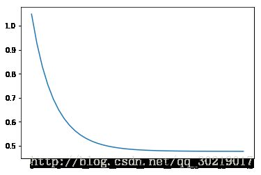

4.scikit-learn中的线性模型

from sklearn import linear_model
from sklearn.preprocessing import StandardScaler

scaler = StandardScaler()
scaler.fit(data)

data_norm = scaler.transform(data)
print(data_norm)

查看scaler缩放后的数据:

array([[ 0.18564659, -0.38900304, -0.48071521, -1.441423  ],
       [ 0.36597354, -1.41593821, -0.72592996, -1.33435646],
       [-0.35533425, -1.41593821, -1.33896682, -0.70095235],
       ..., 
       [-0.1750073 , -1.21055117, -0.45242121, -1.71614797],
       [ 0.00531965,  0.22715806, -0.99943871, -0.60125679],
       [-0.71598815, -0.90247062,  0.4954281 , -1.00253766]])

可以看到，这和我们自己写的缩放的效果是一摸一样的
再查看样本矩阵:

Samples = data_norm[:, 1:]
print(Samples)

结果:

array([[-0.38900304, -0.48071521, -1.441423  ],
       [-1.41593821, -0.72592996, -1.33435646],
       [-1.41593821, -1.33896682, -0.70095235],
       ..., 
       [-1.21055117, -0.45242121, -1.71614797],
       [ 0.22715806, -0.99943871, -0.60125679],
       [-0.90247062,  0.4954281 , -1.00253766]])

再检查结果向量:

Labels = data_norm[:, 0:1]
Labels.shape

(1000, 1)

接下来获取训练集与测试集的训练矩阵和结果向量:

trainX = Samples[:700]
trainY = Labels[:700]

testX = Samples[700:]
testY = Labels[700:]

训练一波模型:

model = linear_model.LinearRegression()
model.fit(trainX, trainY)

训练出来的是一个LinearRegression对象:

LinearRegression(copy_X=True, fit_intercept=True, n_jobs=1, normalize=False)

接下来在测试集上预测一波，再查看预测值和真实值的均方误差(mean squared error):

from sklearn.metrics import mean_squared_error

result = model.predict(testX)

predict_y = scaler.inverse_transform(np.concatenate([result, testX], axis=1))[:, 0]
print(mean_squared_error(predict_y, testY))

1.06594865536

大功告成

5.总结及了解扩展内容

1.从回归算法上:

• 带L2正则的Ridge Regression
• 带L1正则的Lasso Regression

2.扩展为分类

• LDA (Linear Discriminant Analysis)
• 二分类
• 多分类 (根据不同的分类策略)
  
  • OvO (One vs One)
  • OvR (One vs Rest)
  • MvM (Many vs Many)
  • ECOC (Error Correct Output Code)

小小的线性模型，也能有这么多的内容。。。这只是革命第一步

注: 文中所有代码与数据下载地址:https://github.com/NileZhou/ML