The GAN Landscape: Losses, Architectures, Regularization, and Normalization

The GAN Landscape: Losses, Architectures, Regularization, and Normalization

Karol Kurach, Mario Lucic, Xiaohua Zhai, Marcin Michalski, Sylvain Gelly

Abstract

GAN: successful; notoriously challenging to train, requires a significant amount of hyperparameter tuning, neural architecture engineering, and a non-trivial amount of “tricks”
lack of a measure to quantify the failure modes ⇒ ⇒ a plethora of proposed losses, regularization and normalization schemes, and neural architectures
所以本文针对这4个变量进行测试，看看那些情况下能改善训练效果

Introduction

GAN: learning a target distribution, generator + discriminator
contribution:
provide a thorough empirical analysis of (those loss functions, regularization and normalization schemes, coupled with neural architecture choices), and help the researchers and practitioners navigate this space
1. GAN landscape – the set of loss functions, normalization and regularization schemes, and the most commonly used architectures（其实就是4个可控变量） ⇒ ⇒ the non-saturating loss is sufficiently stable across data sets, architectures and hyperparameters
2. decompose the effect of various normalization and regularization schemes, as well as varying architectures ⇒ ⇒ both gradient penalty as well as spectral normalization are useful in the context of high-capacity architectures ⇒ ⇒ simultaneous regularization and normalization are beneficial
3. a discussion of common pitfalls, reproducibility issues, and practical considerations
code and pretrained model

The GAN Landscape

Loss Functions

P,Q P , Q : the target (true) distribution and the model distribution

type	principle	discriminator	generator	form
original GAN	the minimax GAN and the non-saturating (NS) GAN	minimizes the negative log-likelihood for the binary classification task (i.e. is the sample true or fake),is equivalent to minimizing the Jensen-Shannon (JS) divergence between P P and Q Q	maximizes the probability of generated samples being real	LD=Ex∼P(−logD(x))+Ex^∼Q(log(1−D(x^))),LG=Ex^∼Q(−logD(x^)) L D = E x ∼ P ( − log ⁡ D ( x ) ) + E x ^ ∼ Q ( log ⁡ ( 1 − D ( x ^ ) ) ) , L G = E x ^ ∼ Q ( − log ⁡ D ( x ^ ) )
Wasserstein GAN(WGAN)	minimize the Wasserstein distance between P P and Q Q	ensure a 1-Lipschitz discriminator due to exploited Kantorovich-Rubenstein duality ⇒ ⇒ the discriminator weights are clipped to a small absolute value	under an optimal discriminator, minimizing the value function with respect to the generator minimizes the Wasserstein distance between P P and Q Q	LD=Ex^∼Q(D(x^))−Ex∼P(D(x)),LG=−Ex^∼Q(D(x^)) L D = E x ^ ∼ Q ( D ( x ^ ) ) − E x ∼ P ( D ( x ) ) , L G = − E x ^ ∼ Q ( D ( x ^ ) )
least-squares loss (LSGAN)	minimizing the Pearson χ2 χ 2 divergence between P P and Q Q ,is smooth and saturates slower than the sigmoid cross-entropy loss of the JS formulation			LD=Ex^∼Q(D(x^)2)−Ex∼P((1−D(x))2),LG=−Ex^∼Q((1−D(x))2) L D = E x ^ ∼ Q ( D ( x ^ ) 2 ) − E x ∼ P ( ( 1 − D ( x ) ) 2 ) , L G = − E x ^ ∼ Q ( ( 1 − D ( x ) ) 2 )

Regularization and Normalization of the Discriminator

Gradient norm penalty for WGAN: a soft penalty for the violation of 1-Lipschitzness (WGAN GP)

method	gradient evaluation method	drawback
WGAN-GP	on a linear interpolation between training points, generating samples as a proxy to the optimal coupling	depend on the model distribution Q Q which changes during training
DRAGAN	around the data manifold which encourages the discriminator to be piece-wise linear in that region	unclear how to exactly define the manifold

the gradient norm penalty can be considered purely as a regularizer for the discriminator and it was shown that it can improve the performance for other losses, not only the WGAN; the penalty can be scaled by the “confidence” of the discriminator in the context of f-divergences
computing the gradient norms implies a non-trivial running time penalty – essentially doubling the running time

Discriminator normalization:

perspective	benefits	techniques
optimization	more efficient gradient flow, a more stable optimization	Batch normalization(BN),normalizes the pre-activations of nodes in a layer to mean β β and standard deviation γ γ ; Layer normalization (LN), all the hidden units in a layer share the same normalization terms γ γ and β β , but different samples are normalized differently
representation	normailization on spectral structure of weights enhance the representation richness of the layers	spectral normalization: dividing each weight matrix, including the matrices representing convolutional kernels, by their spectral norm. This results in discriminators of higher rank, and guarantees 1-Lipschitzness for linear layers and ReLu activation units, but not the spectral norm of the convolutional mapping

Generator and Discriminator Architecture

DCGAN( + spectral nomalization → → SNDCGAN)
ResNet

Evaluation Metrics

name	principle	method	advantage	drawback
Inception Score (IS)	the conditional label distribution of samples containing meaningful objects should have low entropy, the variability of the samples should be high 越大越好	IS=expEx∼Q(dKL(p(y|x),p(y))) I S = exp ⁡ E x ∼ Q ( d K L ( p ( y | x ) , p ( y ) ) )	well correlated with scores from human annotators	insensitivity to the prior distribution over labels, not being a proper distance
Frechet Inception Distance (FID)	embed samples from P P and Q Q to a feature space with InceptionNet; estimate the mean and variance assuming each embedded data follow a multivariabte Gaussian distribution; compute the Frechet distance between P P and Q Q 越小越好	FID=∥μx−μy∥22+tr(Σx+Σy−2(ΣxΣy)12) F I D = ‖ μ x − μ y ‖ 2 2 + tr ( Σ x + Σ y − 2 ( Σ x Σ y ) 1 2 )	consistent with human judgment and more robust to noise than IS; sensitive to the visual quality of generated samples; can detect intra-class mode dropping
Multi-scale Structural Similarity for Image Quality (MS-SSIM) and Diversity	mode collapse and mode-dropping – failing to capture a mode, or low diversity of generated samples from a given mode measuring the similarity of two images where higher MS-SSIM score indicates more similar images			we do not know the class corresponding to the generated sample the diversity should only be taken into account together with the FID and IS metrics

前两个在SAGAN论文中用到过

Data Sets

CIFAR10, CELEBA-HQ-128, and LSUN-BEDROOM
randomly partition the images into a train, and a test set of 30588 images

Exploring the GAN Landscape

控制变量法
losses + normalization + regularization schemes + architectures

Results and Discussion

4 major components: loss, architecture, regularization, normalization
控制变量法：keep some dimensions fixed, and vary the others

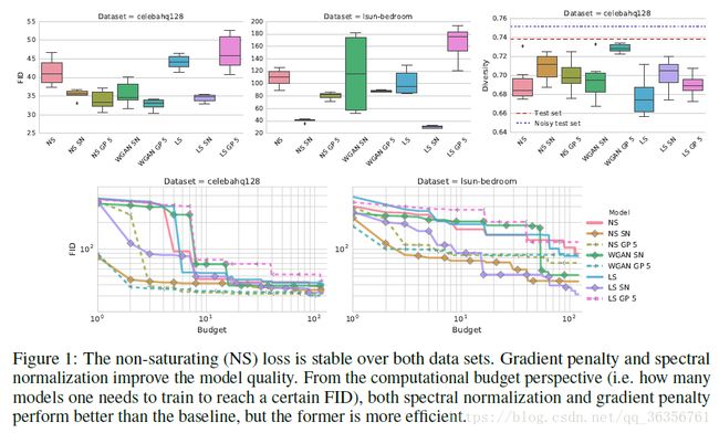
Impact of the Loss Function

the non-saturating loss (NS), the least-squares loss (LS), or the Wasserstein loss (WGAN)

1. the non-saturating loss is stable over both data sets
2. Spectral normalization improves the quality of the model on both data sets
3. gradient penalty can help improve the quality of the model
4. finding a good regularization tradeoff is non-trivial and requires a high computational budget

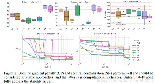
Impact of Regularization and Normalization

Batch normalization (BN), Layer normalization (LN), Spectral normalization (SN), Gradient penalty (GP), Dragan penalty (DR), or L2 regularization

1. adding batch norm to the discriminator hurts the performance
2. gradient penalty can help, but it doesn’t stabilize the training
3. Spectral normalization helps improve the model quality and is more computationally efficient than gradient penalty
4. running the optimization procedure for an additional 100K steps is likely to increase the performance of the models with GP penalty

additional regularization and normalization is benefitial

Impact of Generator and Discriminator Architectures

Resnet, DCGAN

Common Pitfalls

Metrics: how the FID score is computed is not determined…FID should be computed with respect to the test data set and use 10000 test samples and 10000 generated samples on CIFAR10 and LSUN-BEDROOM, and 3000 vs 3000 on CELEBA-HQ-128
Details of neural architectures:
Data sets: data set processing
Implementation details and non-determinism: the mismatch between the algorithm presented in a paper and the code provided online（呵呵…）; there is an embarrassingly large gap between a good implementation and a bad implementation of a given model; removing randomness from the training process

Related Work

Conclusion

所以本文实际上就是对于几个变量进行了测试，得到了几个特定条件下的经验性结论（在其他的框架下不一定有效），纯粹的实验性研究。。。

故弄玄虚，东打一枪西方一炮，逻辑连贯性较弱，读完不知所云。。。