tensorflow个人学习笔记（一）

#tensorflow个人学习笔记（一）
#模块化神经网络的基本结构

###一、生成数据集

opt4_8_generateds.py

#coding:utf-8
#模块化神经网络的结构分为三部分，第一部分生成模拟数据集，在实际应用中，应该是整理数据集
#生成模拟数据集
import numpy as np #引入np模块
import matplotlib.pyplot as plt #引入plt模块
seed = 2 #设定随机种子

def generateds(): #基于seed产生随机数
	rdm = np.random.RandomState(seed)
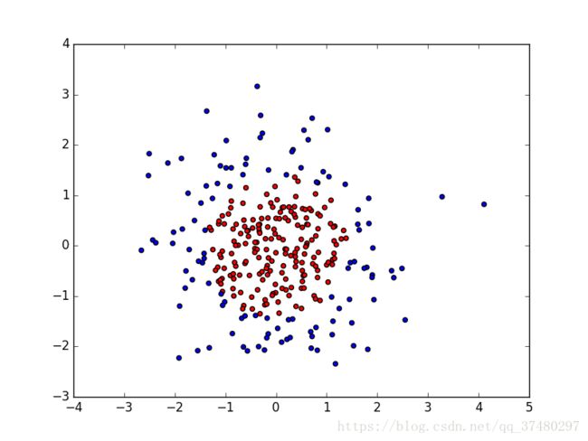
	#随机数返回300行2列的矩阵，表示300组坐标点（x0,x1）作为输入数据集
	X = rdm.randn(300,2)
	#从X这个300行2列的数据集中取出一行，判断两坐标平方和小于2则给Y赋值为1，其余为0
	#最为输入数据集的标签（正确答案）
	Y_ = [int(x0*x0 + x1*x1 < 2) for (x0,x1) in X] #Y_是一个列表，元素是300个1或0
	#遍历Y中的每一个元素，1赋值'red'，其余赋值'blue'，这样可视化显示时，人可以肉眼直观区分
	Y_c= [['red' if y else 'blue'] for y in Y_] #Y_c是一个，列表，其中的元素是['blue']或['red']
	#对数据集X和标签Y进行形状整理，第一个元素为行，第二个元素表示多少列，显然X为两列，Y为一列
	#-1表示未知
	X  = np.vstack(X ).reshape(-1,2) #先纵向堆放，然后在行数未知的情况下，把X整理成2列
	Y_ = np.vstack(Y_).reshape(-1,1) #先纵向堆放，然后在行数未知的情况下，把Y_整理出1列

	return X,Y_,Y_c #X是300行2列的矩阵，Y_是一个1、0列表，Y_c是['blue'],['red']列表

	#print X
	#print Y_
	#print Y_c
	#用plt.scatter画出数据集X各行第0列元素和第1列元素的点即各行的（x0,x1），用各行Y_c对应的值表示颜色（c是colcour）
	#plt.scatter(X[:,0],X[:,1],c=np.squeeze(Y_c))
	#plt.show()
#vstack 是为了沿数数值方向将矩阵堆叠，列数必须一致
#reshape是在不改变数值的前提下改变矩阵的形状 -1表示未知、缺省

###二、定义前向传播

opt4_8_forward.py

#coding:utf-8

#定义神经网络输入、参数和输出，定义前向传播过程
import tensorflow as tf #引入tf模块

def get_weight(shape,regularizer): #定义权重参数
	w = tf.Variable(tf.random_normal(shape),dtype=tf.float32)
	tf.add_to_collection('losses',tf.contrib.layers.l2_regularizer(regularizer)(w))
	return w

def get_bias(shape):
	b = tf.Variable(tf.constant(0.01, shape=shape))
	return b

def forward(x,regularizer): #这个函数构建了神经网络结构
	
	w1 = get_weight([2,11],regularizer)
	b1 = get_bias([11])
	y1 = tf.nn.relu(tf.matmul(x,w1)+b1) #激活函数，使矩阵的每一行的小于0的元素置0

	w2 = get_weight([11,1],regularizer)
	b2 = get_bias([1])
	y  = tf.matmul(y1,w2) + b2 #输出层不激活
	
	return y

###三、定义反向传播过程

opt4_8_backward.py

#coding:utf-8

#引入各个模块
import tensorflow as tf
import numpy as np
import matplotlib.pyplot as plt
import opt4_8_generateds
import opt4_8_forward


#定义超参数 超参数是指学习之前定义的参数，而不是学习时运算得到的参数
STEPS = 40000 #训练40000轮
BATCH_SIZE = 30 #每次给神经网络喂入30个数据
LEARNING_RATE_BASE = 0.001
LEARNING_RATE_DECAY= 0.999
REGULARIZER = 0.01

def backward():
	x = tf.placeholder(tf.float32, shape=(None,2))
	y_= tf.placeholder(tf.float32, shape=(None,1))

	X,Y_,Y_c = opt4_8_generateds.generateds()
	y = opt4_8_forward.forward(x, REGULARIZER)

	#定义global_step
	global_step = tf.Variable(0,trainable=False)
	#定义指数衰减学习率
	learning_rate = tf.train.exponential_decay(
		LEARNING_RATE_BASE,
		global_step,
		300/BATCH_SIZE,
		LEARNING_RATE_DECAY,
		staircase = True)

	#定义损失函数，使用均方误差
	loss_mse = tf.reduce_mean(tf.square(y-y_))
	loss_total = loss_mse + tf.add_n(tf.get_collection('losses'))

	#定义反向传播方法：包含正则化
	train_step = tf.train.AdamOptimizer(learning_rate).minimize(loss_total)

	with tf.Session() as sess:
		init_op = tf.global_variables_initializer() #初始化所有变量
		sess.run(init_op)
		for i in range(STEPS): #使用for循环迭代STEPS轮
			start = (i*BATCH_SIZE) % 300
			end = start + BATCH_SIZE
			sess.run(train_step, feed_dict={x:X[start:end],y_:Y_[start:end]})
			if i % 2000 == 0: #每2k轮打印一次loss值
				loss_v = sess.run(loss_total, feed_dict={x:X,y_:Y_})
				print("After %d steps, loss is : %f" %(i, loss_v))


		xx,yy = np.mgrid[-3:3:.01, -3:3:.01] #在-3与+3之间，以0.01为间距，生成网格坐标点，组成xx,yy坐标集
		grid = np.c_[xx.ravel(), yy.ravel()]
		probs= sess.run(y, feed_dict={x:grid}) #把xx,yy坐标集命名为grid,并喂入神经网络
		probs= probs.reshape(xx.shape) #整理形状，命名为probs

	plt.scatter(X[:,0], X[:,1], c=np.squeeze(Y_c)) #画出离散点
	plt.contour(xx, yy, probs, levels = [.5]) #画出probs为0.5的曲线
	plt.show() #展示图表

if __name__ == '__main__' :
	backward()

###输出结果

After 0 steps, loss is : 15.128757
After 2000 steps, loss is : 0.263676
After 4000 steps, loss is : 0.181108
After 6000 steps, loss is : 0.145825
After 8000 steps, loss is : 0.116128
After 10000 steps, loss is : 0.099375
After 12000 steps, loss is : 0.095520
After 14000 steps, loss is : 0.095004
After 16000 steps, loss is : 0.093543
After 18000 steps, loss is : 0.092141
After 20000 steps, loss is : 0.091536
After 22000 steps, loss is : 0.091219
After 24000 steps, loss is : 0.091075
After 26000 steps, loss is : 0.090997
After 28000 steps, loss is : 0.090936
After 30000 steps, loss is : 0.090890
After 32000 steps, loss is : 0.090851
After 34000 steps, loss is : 0.090831
After 36000 steps, loss is : 0.090816
After 38000 steps, loss is : 0.090807
/home/lixiang/.local/lib/python2.7/site-packages/numpy/ma/core.py:6447: MaskedArrayFutureWarning: In the future the default for ma.maximum.reduce will be axis=0, not the current None, to match np.maximum.reduce. Explicitly pass 0 or None to silence this warning.
  return self.reduce(a)
/home/lixiang/.local/lib/python2.7/site-packages/numpy/ma/core.py:6447: MaskedArrayFutureWarning: In the future the default for ma.minimum.reduce will be axis=0, not the current None, to match np.minimum.reduce. Explicitly pass 0 or None to silence this warning.
  return self.reduce(a)