CS224n Assignment 1

https://web.stanford.edu/class/archive/cs/cs224n/cs224n.1174/syllabus.html 第一次作业笔记

Softmax

softmax常数不变性

由于，因此多余的可以上下消除，于是：
这里

发现了一个Softmax非常好的性质，即使两个数都很大比如 1000与 1001，其结果与 1和2的结果相同，即其只关注数字之间的差，而不是差占的比例。

Python实现

之所以介绍Softmax常数不变性，是因为发现给定的测试用例非常大，直接计算次方

import numpy as np


def softmax(x):
    orig_shape = x.shape

    if len(x.shape) > 1:
        # Matrix
        ### YOUR CODE HERE
        x_max = np.max(x, axis=1).reshape(x.shape[0], 1)
        x -= x_max
        exp_sum = np.sum(np.exp(x), axis=1).reshape(x.shape[0], 1)
        x = np.exp(x) / exp_sum 
        ### END YOUR CODE
    else:
        # Vector
        ### YOUR CODE HERE
        x_max = np.max(x)
        x -= x_max
        exp_sum = np.sum(np.exp(x))
        x = np.exp(x) / exp_sum
        ### END YOUR CODE
        #or:  x = (np.exp(x)/sum(np.exp(x)))   

    assert x.shape == orig_shape
    return x

def test_softmax_basic():
    """
    Some simple tests to get you started.
    Warning: these are not exhaustive.
    """
    print("Running basic tests...")
    test1 = softmax(np.array([1,2]))
    print(test1)
    ans1 = np.array([0.26894142,  0.73105858])
    assert np.allclose(test1, ans1, rtol=1e-05, atol=1e-06)

    test2 = softmax(np.array([[1001,1002],[3,4]]))
    print(test2)
    ans2 = np.array([
        [0.26894142, 0.73105858],
        [0.26894142, 0.73105858]])
    assert np.allclose(test2, ans2, rtol=1e-05, atol=1e-06)

    test3 = softmax(np.array([[-1001,-1002]]))
    print(test3)
    ans3 = np.array([0.73105858, 0.26894142])
    assert np.allclose(test3, ans3, rtol=1e-05, atol=1e-06)

    print("You should be able to verify these results by hand!\n")

if __name__ == "__main__":
    test_softmax_basic()

神经网络基础

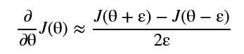
梯度检查

image

Sigmoid导数

定义如下，发现。

image

即:

交叉熵定义

当使用交叉熵作为评价指标时，求梯度：

• 已知:
• 交叉熵：

其中是指示变量，如果该类别和样本的类别相同就是1，否则就是0。因为y一般为one-hot类型。

而 表示每种类型的概率，概率已经过softmax计算。

对于交叉熵其实有多重定义的方式，但含义相同：

分别为：

二分类定义

• y——表示样本的label，正类为1，负类为0
• p——表示样本预测为正的概率

多分类定义

• y——指示变量（0或1）,如果该类别和样本的类别相同就是1，否则是0；
• p——对于观测样本属于类别c的预测概率。

但表示的意思都相同，交叉熵用于反映 分类正确时的概率情况。

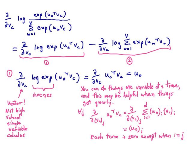
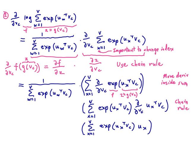
Softmax导数

进入解答：

• 首先定义和分子分母。

• 对求导：

  

注意: 分子是 ，分母是所有的 ，而求偏微的是 。

• 因此，根据i与j的关系，分为两种情况：

• 当 时：

$f_i' = e^{\theta_i}$,$g_i' = e^{\theta_j}$ 



$\begin{align} \frac{\partial{S_i}}{\partial{\theta_j}} &=\frac{e^{\theta_i}\sum^{k}_{k=1}e^{\theta_k} - e^{\theta_i}e^{\theta_j}}{(\sum^{k}_{k=1}e^{\theta_k})^2} \\ &= \frac{e^{\theta_{i}}}{\sum_{k} e^{\theta_{k}}} \times \frac{\sum_{k} e^{\theta_{k}} – e^{\theta_{j}}}{\sum_{k} e^{\theta_{k}}} \nonumber \\  &= S_{i} \times (1 – S_{i})   \end{align}$

• 当时：

$f'_{i} = 0 $,$g'_{i} = e^{\theta_{j}}$ 



$\begin{align}  \frac{\partial{S_i}}{\partial{\theta_j}} &= \frac{0 – e^{\theta_{j}} e^{\theta_{i}}}{(\sum_{k} e^{\theta_{k}})^{2}}  \\&= – \frac{e^{\theta_{j}}}{\sum_{k} ^{\theta_{k}}} \times \frac{e^{\theta_{i}}}{\sum_{k} e^{\theta_{k}}} \\ &=-S_j \times S_i\end{align}$

交叉熵梯度

计算 ，根据链式法则，

$\begin{align}      \frac{\partial CE}{\partial \theta_{i}} &= – \sum_{k} y_{k} \frac{\partial log S_{k}}{\partial \theta_{i}}  \\&= – \sum_{k} y_{k} \frac{1}{S_{k}} \frac{\partial S_{k}}{\partial \theta_{i}} \\ &= – y_{i} (1 – S_{i}) – \sum_{k \ne i} y_{k} \frac{1}{S_{k}} (-S_{k} \times S_{i}) \\ &= – y_{i} (1 – S_{i}) + \sum_{k \ne i} y_{k} S_{i} \\ &= S_{i}(\sum_{k} y_{k}) – y_{i}\end{align}$

因为，所以

反向传播计算神经网络梯度

根据题目给定的定义：

image

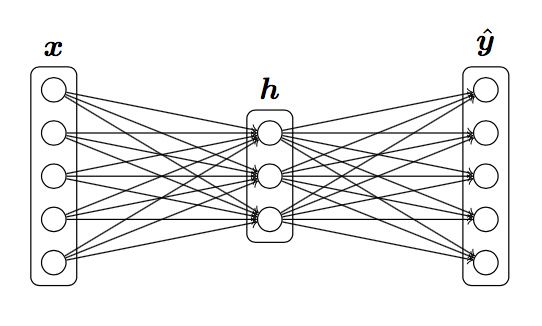
已知损失函数，,

求,,,,

解答：

反向传播，定义， ：

对于输出层来说，的输入为 ，而输出则为

上小节计算得到 的梯度为 ,

可以使用 替代 ，得到

• # 推测这里使用点乘的原因是经过计算后，应该是一个标量，而不是向量。

• 于是得到：

与计算相似，计算

如果仍然对反向传播有疑惑

• 可以参考一文弄懂神经网络中的反向传播法——BackPropagation，画图出来推导一下。

• 如何直观地解释 backpropagation 算法？ - Anonymous的回答 - 知乎
  https://www.zhihu.com/question/27239198/answer/89853077

参数数量

代码实现

• sigmoid和对应的梯度

def sigmoid(x):
    s = 1 / (1 + np.exp(-x))
    return s

def sigmoid_grad(s):
    ds = s * (1-s)
    return ds

• 梯度检查

import numpy as np
import random


# First implement a gradient checker by filling in the following functions
def gradcheck_naive(f, x):
    """ Gradient check for a function f.

    Arguments:
    f -- a function that takes a single argument and outputs the
         cost and its gradients
    x -- the point (numpy array) to check the gradient at
    """

    rndstate = random.getstate()
    random.setstate(rndstate)
    fx, grad = f(x) # Evaluate function value at original point
    h = 1e-4        # Do not change this!

    # Iterate over all indexes in x
    it = np.nditer(x, flags=['multi_index'], op_flags=['readwrite'])
    while not it.finished:
        ix = it.multi_index
        print(ix)
        # Try modifying x[ix] with h defined above to compute
        # numerical gradients. Make sure you call random.setstate(rndstate)
        # before calling f(x) each time. This will make it possible
        # to test cost functions with built in randomness later.

        ### YOUR CODE HERE:
        x[ix] += h
        new_f1 = f(x)[0]
        x[ix] -= 2*h
        random.setstate(rndstate)
        new_f2 = f(x)[0]
        x[ix] += h
        numgrad = (new_f1 - new_f2) / (2 * h)
        ### END YOUR CODE

        # Compare gradients
        reldiff = abs(numgrad - grad[ix]) / max(1, abs(numgrad), abs(grad[ix]))
        if reldiff > 1e-5:
            print("Gradient check failed.")
            print("First gradient error found at index %s" % str(ix))
            print("Your gradient: %f \t Numerical gradient: %f" % (
                grad[ix], numgrad))
            return

        it.iternext() # Step to next dimension

    print("Gradient check passed!")

• 反向传播

  def forward_backward_prop(data, labels, params, dimensions):
      """
      Forward and backward propagation for a two-layer sigmoidal network
      Compute the forward propagation and for the cross entropy cost,
      and backward propagation for the gradients for all parameters.
      Arguments:
      data -- M x Dx matrix, where each row is a training example.
      labels -- M x Dy matrix, where each row is a one-hot vector.
      params -- Model parameters, these are unpacked for you.
      dimensions -- A tuple of input dimension, number of hidden units
                    and output dimension
      """
      ### Unpack network parameters (do not modify)
      ofs = 0
      Dx, H, Dy = (dimensions[0], dimensions[1], dimensions[2])
      W1 = np.reshape(params[ofs:ofs+ Dx * H], (Dx, H))
      ofs += Dx * H
      b1 = np.reshape(params[ofs:ofs + H], (1, H))
      ofs += H
      W2 = np.reshape(params[ofs:ofs + H * Dy], (H, Dy))
      ofs += H * Dy
      b2 = np.reshape(params[ofs:ofs + Dy], (1, Dy))
      ### YOUR CODE HERE: forward propagation
      h = sigmoid(np.dot(data,W1) + b1)
      yhat = softmax(np.dot(h,W2) + b2)
      ### END YOUR CODE
      ### YOUR CODE HERE: backward propagation
      cost = np.sum(-np.log(yhat[labels==1])) 
      
      d1 = (yhat - labels)
      gradW2 = np.dot(h.T, d1)
      gradb2 = np.sum(d1,0,keepdims=True)
      
      d2 = np.dot(d1,W2.T)
      # h = sigmoid(z_1)
      d3 = sigmoid_grad(h) * d2
      gradW1 = np.dot(data.T,d3)
      gradb1 = np.sum(d3,0)
      
      ### END YOUR CODE
      ### Stack gradients (do not modify)
      grad = np.concatenate((gradW1.flatten(), gradb1.flatten(),
          gradW2.flatten(), gradb2.flatten()))
      return cost, grad

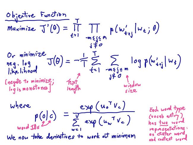
word2vec

关于词向量的梯度

在以softmax为假设函数的word2vec中

是中央单词的词向量

() 是第 个词语的词向量。

假设使用交叉熵作为损失函数， 为正确单词 (one-hot向量的第 维为1)，请推导损失函数关于的梯度。

提示：

其中 = ,,, 是所有词向量构成的矩阵。

解答：

首先明确本题给定的模型是skip-gram ，通过给定中心词，来发现周围词的。

定义 ， 表示所有词向量组成的矩阵，而 也表示的是一个词向量。

hint: 如果两个向量相似性越高，则乘积也就越大。想象一下余弦夹角，应该比较好明白。

因为中所有的词向量，都和乘一下获得。

是干嘛用的呢？ 内就有W个值，每个值表示和 相似程度，通过这个相似度选出最大值，然后与实际对比，进行交叉熵的计算。

已知： 和

因此：

---

除了上述表示之外，还有另一种计算方法

image

image

image

[图片上传失败...(image-53cc75-1557025564256)]

于是：

仔细观察这两种写法，会发现其实是一回事，都是 观察与期望的差()。

推导lookup-table梯度

与词向量相似

负采样时的梯度推导

假设进行负采样，样本数为，正确答案为，那么有。负采样损失函数定义如下：

其中：

解答：

首先说明一下，从哪里来的，参考note1 第11页，会有一个非常详细的解释。

全部梯度

推导窗口半径的上下文[word ,...,word ,word ,word ,...,word ]时，skip-gram 和 CBOW的损失函数 ( 是正确答案的词向量）或说 或 关于每个词向量的梯度。

对于skip-gram来讲，的上下文对应的损失函数是：

这里  是离中心词距离的那个单词。

而CBOW稍有不同，不使用中心词而使用上下文词向量的和作为输入去预测中心词：

然后CBOW的损失函数是：

解答：

根据前面的推导，知道如何得到梯度和。那么所求的梯度可以写作：

skip-gram

CBOW

补充部分：

• 矩阵的每个行向量的长度归一化

   x = x/np.linalg.norm(x,axis=1,keepdims=True)
  

• 在斯坦福情感树库上训练词向量

  直接运行q3_run即可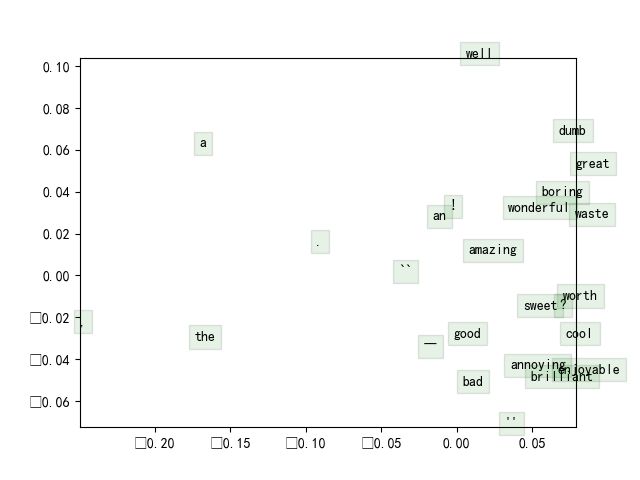

  

  image

情感分析

特征向量

最简单的特征选择方法就是取所有词向量的平均

    sentence_index = [tokens[i] for i in sentence]
    for index in sentence_index:
        sentVector += wordVectors[index, :]

    sentVector /= len(sentence)

正则化

values = np.logspace(-4, 2, num=100, base=10)

调参

bestResult = max(results, key= lambda x: x['dev'])

惩罚因子对效果的影响

image

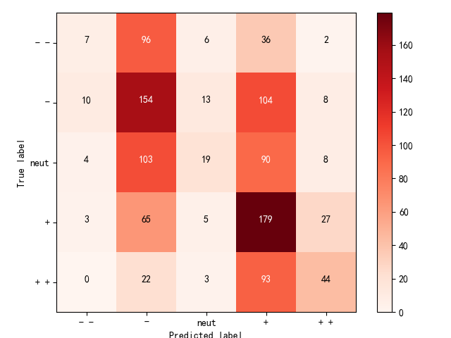
confusion matrix

关联性排序的一个东西，对角线上的元素越多，预测越准确。

image