《三天搞定Python基础概念之第二天》中文版

Day2，即第二篇主要是讲一些偏计算的Library的使用，也就是numpy，scipy，sympy和matplotlib。

前言：
首先，非常感谢Jiang老师将其分享出来！本课件非常经典！
经过笔者亲测，竟然确实只要三天，便可管中窥豹洞见Python及主要库的应用。实属难得诚意之作！
其次，只是鉴于Jiang老师提供的原始课件用英文写成，而我作为Python的爱好者计算机英文又不太熟练，讲义看起来比较慢，为了提高自学课件的效率，故我花了点时间将其翻译成中文，以便将来自己快速复习用。
该版仅用于个人学习之用。
再次，译者因工作中需要用到数据分析、风险可视化与管理，因此学习python，翻译水平有限，请谅解。
在征得原作者Yupeng Jiang老师的同意后，现在我将中文版本分享给大家。

作者：Dr.Yupeng Jiang

• 伦敦大学学院 数学系 (全球顶尖大学，世界排名第7 《2018QS世界大学排名》，英国第3名)
• 2016年6月5日
• [原版课件来自] https://zhuanlan.zhihu.com/p/21332075
• [中文版的说明] https://zhuanlan.zhihu.com/p/29184240

翻译：Murphy Wan

大纲（ Outline）

• 第1天：Python和科学编程介绍。 Python中的基础知识：

  • 数据类型
  • 控制结构
  • 功能
  • I/O文件

• 第2天：用Numpy，Scipy，Matplotlib和其他模块进行计算。 用Python解决一些数学问题。

• 第3天：时间序列：用Pandas进行统计和实际数据分析。 随机和蒙特卡罗。

------------------------------以下为英文原文-------------------------------------

• Day 1: Introduction to Python and scientific programming. Basics in Python: data type, contro structures, fu nctions, l/O file.
• Day 2: Computation with Numpy, Scipy, Matplotlib and other modules. Solving some maths problems with Python.
• Day 3: Time series: statistics and real data analysis with Pandas. Stochastics and Monte Carlo.

第二天的内容

Import modules

Numpy

Scipy

Matplotlib

Sympy

导入模块 (Import modules)

• 可以通过输入import关键字来导入模块

import numpy

• 或者使用简称，即将模块通过as关键字来命名一个简称

import numpy as np

• 有时您不必导入整个模块，就像下面一样：

from scipy.stats import norm

------------------------------以下为英文原文-------------------------------------

• One can import a module by typing

import numpy

• or for short by

2import numpy as np

• Sometimes you do not have to import the whole module, like

from scipy.stats import norm

练习 (Exercise)

• 尝试导入模块时间，并使用它来获取计算机运行特定代码所需的时间。

import timeit
def funl (x, y):      
     return x**2 + y**3

t_start  =  timeit.default_timer()
z =  funl(109.2, 367.1)
t_end  =   timeit.default_timer()

cost  =  t_end -t_start
print ( 'Time cost of funl is  %f' %cost)

------------------------------以下为英文原文-------------------------------------

• Try to import the module timeit and use it to obtain how long you computer takes to run a specific code.

import timeit
def  funl (x, y):      
return x**2 + y**3
t_start  =  timeit.default_timer()
z =  funl(109.2, 367.1)
t_end  =   timeit.default_timer()
cost  =  t_end -t_start
print ( 'Time cost of funl is  %f' %cost)

我们会遇到的模块

• NumPy：多维数组的有效操作。 高效的数学函数。

• Matplotlib：可视化：2D和（最近）3D图

• SciPy：大型库实现各种数值算法，例如：

  • 线性和非线性方程的解
  • 优化
  • 数值整合

• Sympy：符号计算（解析的 Analytical）

• Pandas：统计与数据分析（明天）

------------------------------以下为英文原文-------------------------------------

Modules we will encounter

• NumPy: Efficient manipulation of multidimensional arrays. Efficient mathematical functions.
• Matplotlib: Visualisations: 2D and (recently) 3D plots
• SciPy: Large library implementing various numerical algorithms, e.g.:
  • solution of linear and nonlinear equations
  • optimisation
  • numerical integration
• Sympy: Symbolic computation (Analytical).
• Pandas: Statistical and data analysis(tomorrow)

Numpy

ndarray类型

• NumPy提供了一种新的数据类型：ndarray（n维数组）。
  • 与元组和列表不同，数组只能存储相同类型的对象（例如只有floats或只有ints）
  • 这使得数组上的操作比列表快得多; 此外，数组占用的内存少于列表。
  • 数组为列表索引机制提供强大的扩展。

------------------------------以下为英文原文-------------------------------------

The ndarray type

• NumPy provides a new data type: ndarray (n-dimensional array).

  • Unlike tuples and lists, arrays can only store objects of the same type (e.g. only floats or only ints)
  • This makes operations on arrays much faster than on lists; in addition, arrays take less memory than lists.
  • Arrays provide powerful extensions to the list indexing mechanism.

创建ndarray

• 我们导入Numpy（在脚本的开头或终端）：

import numpy as np

• 然后我们创建numpy数组：

In [1] : np.array([2, 3, 6, 7])   
Out[l] : array([2, 3, 6, 7])   
In [2] : np.array([2, 3, 6, 7.])   
Out [2] :  array([ 2.,  3.,  6., 7.])  <- Hamogenaous   
In  [3] :  np.array( [2,  3,  6,  7+1j])   
Out [3] :  array([ 2.+0.j,  3.+0.j,  6.+0.j,  7.+1.j])

------------------------------以下为英文原文-------------------------------------

Create the ndarray

• We import Numpy (at the beginning of the script or in the terminal):

import numpy as np

• Then we create numpy arrays:

In [1] : np.array([2, 3, 6, 7])   
Out[l] : array([2, 3, 6, 7])   
In [2] : np.array([2, 3, 6, 7.])   
Out [2] :  array([ 2.,  3.,  6., 7.])  <- Hamogenaous   
In  [3] :  np.array( [2,  3,  6,  7+ij])   
Out [3] :  array([ 2.+0.j,  3.+0.j,  6.+0.j,  7.+1.j])

创建均匀间隔的数组

• arange：

in[1]：np.arange（5）
Out [l]：array（[0，1，2，3，4]）

range(start, stop, step)的所有三个参数即起始值，结束值，步长都是可以用的 另外还有一个数据的dtype参数

  in[2]：np.arange（10，100，20，dtype = float）
  Out [2]：array（[10.，30.，50.，70.，90.]）

• linspace（start，stop，num）返回数字间隔均匀的样本，按区间[start，stop]计算：

  in[3]：np.linspace（0.，2.5，5）         
  Out [3]：array([0.，0.625，1.25，1.875，2.5])
  

这在生成plots图表中非常有用。

• 注释：即从0开始，到2.5结束，然后分成5等份

多维数组矩阵 (Matrix by multidimensional array)

In [1] : a = np.array([[l, 2, 3]  [4, 5, 6]])
                          ^ 第一行 (Row 1)
In  [2] : a
Out [2] : array([[l, 2,  3] ,   [4,  5,  6]])

In  [3] : a.shape  #<- 行、列数等 (Number of rows, columns etc.)
Out [3] : (2,3)

In  [4] : a.ndim   #<- 维度数  (Number of dimensions)
Out [4] : 2

In  [5] : a,size   #<- 元素数量 (Total number of elements)
Out [5] : 6

形状变化 (Shape changing)

import numpy as np

a = np .arange(0, 20, 1) ＃1维
b = a.reshape((4, 5))   ＃4行5列
c = a.reshape((20, 1))  ＃2维
d = a.reshape((-1, 4))  ＃-1：自动确定
＃a.shape =(4, 5) ＃改变a的形状

Size（N，），（N，1）和（1，N）是不同的!!!

• Size（N, ）表示数组是一维的。
• Size（N，1）表示数组是维数为2, N列和1行。
• Size（1，N）表示数组是维数为2, 1行和N列。

让我们看一个例子,如下

例子 (Example)

import numpy as np

a = np.array([1,2,3,4,5])
b = a.copy ()

c1 =  np.dot(np.transpose(a), b)
print(c1)
c2  = np.dot(a, np.transpose(b))
print(c2)

ax  =  np.reshape(a, (5,1))
bx  =  np.reshape(b, (1,5))
c = np.dot(ax, bx)
print(c)

使用完全相同的元素填充数组 (Filling arrays with identical elements)

In [1] : np.zeros(3)              # zero(),全0填充数组
Out[l] : array([ 0., 0., 0.])

In [2] : np.zeros((2, 2), complex)
Out[2] : array([[ 0.+0.j, 0.+0.j],                
                [ 0.+0.j, 0.+0.j]])

In [3] : np.ones((2, 3))          # ones(),全1填充数组
Out[3] : array([[ 1., 1., 1.],
                [ 1., 1., 1.]])

使用随机数字填充数组 (Filling arrays with random numbers)

• rand: 0和1之间均匀分布的随机数 (random numbers uniformly distributed between 0 and 1)

   In [1] : np.random.rand(2, 4)   
   Out[1] : array([[ 0.373767 , 0.24377115, 0.1050342 , 0.16582644] , 
                   [ 0.31149806, 0.02596055, 0.42367316, 0.67975249l])

• randn: 均值为0，标准差为1的标准（高斯）正态分布 {standard normal (Gaussian) distribution with mean 0 and variance 1}

  In [2]: np.random.randn(2, 4)  
  Out[2]: array([[ 0.87747152, 0.39977447, -0.83964985, -1.05129899], 
                 [-1.07933484, 0.49448873,   -1.32648606, -0.94193424]])

• 其他标准分布也可以使用 (Other standard distributions are also available.)

---

数组切片（1D） (Array sliciing(1D))

• 以格式start：stop可以用来提取数组的片段（从开始到不包括stop）

In [77]：a = np.array（[0，1，2，3，4]）
Out[77]：array（[0，1，2，3，4]）

In [78]：a [1：3]        #<--index从0开始 ,所以1是第二个数字，即对应1到3结束，就是到第三个数字，对应是2
Out[78]：array([1，2])

• start可以省略，在这种情况下，它被设置为零(Notes:貌似留空更合适)：

In [79]：a [:3]
Out[79]：array（[0，1，2]）

• stop也可以省略，在这种情况下它被设置为数组长度：

In [80]：a [1：]
Out[80]：array（[1，2，3，4]）

• 也可以使用负指数，具有标准含义：

In [81]：a [1：-1]
Out[81]：array（[1,2,3]）      # <-- stop为-1表示倒数第二个数

---

数组切片（1D）

• 整个数组：a或a [：]

In [77]：a = np.array（[0,1,2,3,4]）
Out[77]：array（[0，1，2，3，4])

• 要获取，例如每个其他元素，您可以在第二个冒号后面指定第三个数字（步骤(step)）：

In [79]：a [：：2]
Out[79]：array（[0，2，4]） 

In [80]：a [1：4：2]
Out[80]：array（[l，3]）

• -1的这个步骤可用于反转数组：

In [81]：a [::-1]
Out[81]：array（[4，3，2，1，0]）

---

数组索引(2D) （Array indexing (2D)）

• 对于多维数组，索引是整数元组：(For multidimensional arrays, indices are tuples of integers:)

In [93] :  a = np.arange(12) ; a.shape =  (3,  4);  a
Out[93] :  array([[0,  1,  2,  3],
                  [4,  5,  6,  7],
                  [8, 9,  10, 11]])

In [94] : a[1,2]
Out[94] : 6

In [95] : a[1,-1]
Out[95] : 7

---

数组切片（2D）：单行和列 (Array slicing (2D): single rows and columns)

• 索引的工作与列表完全相同：（Indexing works exactly like for lists:）

In [96] : a = np.arange(12); a.shape = (3, 4); a   
Out[96] : array([[0, 1, 2, 3],
                 [4, 5, 6, 7],
                 [8, 9,10,11]])

In [97] : a[:,1]
Out[97] : array([1,5,9])

In [98] : a[2,:]
Out[98] : array([ 8, 9, 10, 11])

In [99] : a[1][2]
Out[99] : 6

• 不必明确提供尾随的冒号：（Trailing colons need not be given explicitly:）

In [100] : a[2]
Out[100] : array([8,9,10,11]) 

---

数组索引 (Array indexing)

>>> a[0,3:5]
array( [3,4] )

>>> a[4:,4:]
array([[44, 45], 
       [54, 55]])

>>> a[:,2]
array([2,12,22,32,42,52])

>>> a[2: :2, ::2]
array([[20, 22, 24]       
       [40, 42, 44]])

mofang.jpg

---

副本（copy）和视图（view）

• 采用标准的list切片为其建立副本
• 采用一个NumPy数组的切片可以在原始数组中创建一个视图。 两个数组都指向相同的内存。因此，当修改视图时，原始数组也被修改：

In [30] : a = np.arange(5); a
Out[30] : array([0, 1, 2, 3, 4])

In [31] : b = a[2:]; b
Out[31] : array([2, 3, 4])

In [32] : b[0] = 100
In [33] : b

Out[33] : array([l00, 3, 4])
In [34] : a
Out[34] : array([0,1,100,3,4])

---

副本和视图 (Copies and views)

• 为避免修改原始数组，可以制作一个切片的副本 (To avoid modifying the original array, one can make a copy of a slice:)

In [30] : a = np.arange(5); a
Out[30] : array([0, 1, 2, 3, 4])

In [31] : b = a[2:].copy(); b
Out[31] : array([2, 3, 4])

In [32] : b[0] = 100
In [33] : b
Out[33] : array([100, 3, 4])

In [34] : a 
Out[34] : array([ 0,  1.  2,  3,  4])

---

矩阵乘法 (Matrix multiplication)

• 运算符 * 表示元素乘法，而不是矩阵乘法：(The * operator represents elementwise multiplication , not matrix multiplication:)

In [1]: A = np.array([[1, 2],[3, 4]])
In [2]: A
Out[2]: array([[1, 2],
               [3, 4]])

In [3]: A * A
Out[3]: array([[1, 4],
               [9, 16]])            

• 使用dot（）函数进行矩阵乘法：(Matrix multiplication is done with the dot() function:)

In [4]: np.dot(A, A)
Out[4]: array([[ 7, 10],    
               [15, 22]])  

--

矩阵乘法

• dot（）方法也适用于矩阵向量(matrix-vector)乘法：

In [1]: A
Out[1]: array([[1, 2],[3, 4]])

In [2]: x = np.array([10, 20])
In [3]: np.dot(A, x)
Out[3]: array([ 50, 110])

In [4]: np.dot(x, A)
Out[4]: array([ 70, 100])

---

将数组保存到文件 (Saving arrays to files)

• savetxt()将表保存到文本文件。 (savetxt() saves a table to a text file.)

In  [1]: a = np,linspace(0. 1, 12); a,shape ' (3, 4); a
Out [1] :
array([[ 0.  ,  0.09090909, 0.18181818,  0.27272727],
[  0.36363636,  0.45454545, 0.54545455,  0.63636364],
[  0.72727273,  0.81818182. 0.90909091,  1.]])

In [2] : np.savetxt("myfile.txt", a)

• 其他可用的格式(参见API文档) {Other formats of file are available (see documentation)}

• save()将表保存为Numpy“.npy”格式的二进制文件 (save() saves a table to a binary file in NumPy ".npy" format.)

  - In [3] : np.save("myfile" ,a)    

• 生成一个二进制文件myfile .npy，其中包含一个可以使用np.load（）加载的文件。 {produces a binary file myfile .npy that contains a and that can be loaded with np.load().}

---

将文本文件读入数组 (Reading text files into arrays)

• loadtxt（）将以文本文件存储的表读入数组。 (loadtxt() reads a table stored as a text file into an array.)

• 默认情况下，loadtxt()假定列是用空格分隔的。 您可以通过修改可选的参数进行更改。 以散列（＃）开头的行将被忽略。 (By default, loadtxt() assumes that columns are separated with whitespace. You can change this by modifying optional parameters. Lines starting with hashes (#) are ignored.)

• 示例文本文件data.txt： (Example text file data.txt:)

  |Year| Min temp.| Hax temp.|

  |1990| -1.5 | 25.3|

  |1991| -3.2| 21.2|

• Code:

   In [1] : tabla = np.loadtxt("data.txt")
   In [2] : table
   Out[2] :
   array ([[ 1.99000000e+03,   -1.50000000e+00,   2.53000000e+01],    
   [ 1.9910000e+03,  -3.2000000e+00,  2.12000000e+01]

---

Numpy包含更高效率的功能

• Numpy包含许多常用的数学函数，例如：

  • np.log
  • np.maximum
  • np.sin
  • np.exp
  • np.abs

• 在大多数情况下，Numpy函数比Math包中的类似函数更有效，特别是对于大规模数据。

---

Scipy (库)

SciPy的结构

• scipy.integrate - >积分和普通微分方程
• scipy.linalg - >线性代数
• scipy.ndimage - >图像处理
• scipy.optimize - >优化和根查找(root finding)
• scipy.special - >特殊功能
• scipy.stats - >统计功能
• ...

要加载一个特定的模块，请这样使用, 例如 :

• from scipy import linalg

---

线性代数 (Linearalgebra)

• 线性方程的解 (Solution of linear equations:)

import numpy as np
from scipy import linalg    

A = np.random.randn(5, 5)
b = np.random.randn(5)
x = linalg.solve(A, b)     # A x = b#print(x)    
eigen = linalg.eig(A)     # eigens#print(eigen)    
det = linalg.det(A)     # determinant    
print(det)            

• linalg的其他有用的方法：eig()（特征值和特征向量），det()（行列式）。{Other useful functions from linalg: eig() (eigenvalues and eigenvectors), det() (determinant). }

数值整合 (Numerical integration)

• integration.quad是一维积分的自适应数值积分的函数。 (integrate.quad is a function for adaptive numerical quadrature of one-dimensional integrals.)

import numpy as np
from scipy import integrate

def fun(x):
    return np.log(x)

value, error = integrate.quad(fun,0,1)
print(value)
print(error)

用Scipy进行统计 (Statistics in Scipy)

• scipy具有用于统计功能的子库，您可以导入它 (scipy has a sub-library for statistical functions, you can import it by)

from scipy import stats

• 然后您可以使用一些有用的统计功能。 例如，给出标准正态分布的累积密度函数（Then you are able to use some useful statistical function. For example, the cummulative density function of a standard normal distribution is given like

• 这个包，我们可以直接使用它，如下: （with this package, we can directly use it like)

from scipy import stats
y = stats.norm.cdf(1.2)

---

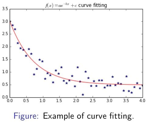
优化：数据拟合 (Optimisation: Data fitting)

import numpy as np
from scipy.optimize import curve_fit
import matplotlib.pyplot as plt

def func(x, a, b, c):    
    return a * np.exp(-b * x) + c

x = np.linspace(0, 4, 50)
y = func(x, 2.5, 1.3, 0.5)
ydata = y+0.2*np.random.normal(size=len(x))
popt, pcov = curve_fit(func, x, ydata)
plt.plot(x, ydata, ’b*’)
plt.plot(x, func(x, popt[0], \ 
                    popt[1], popt[2]), ’r-’)
plt.title(’$f(x)=ae^{-bx}+c$ curve fitting’)

优化:根搜索 (Optimisation: Root searching)

import numpy as np
from scipy import optimize

def fun(x):
    return np.exp(np.exp(x)) - x**2

# 通过初始化点0，找到兴趣0 (find zero of fun with initial point 0)
# 通过Newton-Raphson方法 (by Newton-Raphson)
value1 = optimize.newton(fun, 0)

# 通过二分法找到介于(-5,5)之间的 (find zero between (-5,5) by bisection)
value2 = optimize.bisect(fun, -5, 5)

---

Matplotlib

最简单的制图 (The simplest plot)

• 导入库需要添加以下内容

from matplotlib import pyplot as plt

• 为了绘制一个函数，我们操作如下 (To plot a function, we do:)

import numpy as np
import matplotlib.pyplot as plt

x = np.linspace(0, 10, 201)
#y = x ** 0.5
#plt.plot(x, y) # default plot
plt.figure(figsize = (3, 3)) # new fig
plt.plot(x, x**0.3, ’r--’) # red dashed
plt.plot(x, x-1, ’k-’) # continue plot
plt.plot(x, np.zeros_like(x), ’k-’)

• 注意：您的x轴在plt.plot函数中应与y轴的尺寸相同。 (Note: Your x-axis should be the same dimension to y-axis in plt.plot function.)

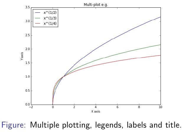
多个制图图例标签和标题 (Multiple plotting, legends, labels and title)

import numpy as np
import matplotlib.pyplot as plt

x = np.linspace(0, 10, 201)
plt.figure(figsize = (4, 4))
for n in range(2, 5):
    y = x ** (1 / n)
    plt.plot(x, y, label=’x^(1/’ \
            + str(n) + ’)’)
plt.legend(loc = ’best’)
plt.xlabel(’X axis’)
plt.ylabel(’Y axis’)
plt.xlim(-2, 10)
plt.title(’Multi-plot e.g. ’, fontsize = 18)

• Forinformations:See

help(plt.plot)  

绘制子图 (Subplots )

import numpy as np’
import matplotlib.pyplot as plt

def pffcall(S, K):    
    return np.maximum(S - K, 0.0)
def pffput(S, K):
    return np.maximum(K - S, 0.0)    

S = np.linspace(50, 151, 100)
fig = plt.figure(figsize=(12, 6))  

sub1 = fig.add_subplot(121)     # col, row, num    
sub1.set_title('Call', fontsize = 18)
plt.plot(S, pffcall(S, 100), 'r-', lw = 4)
plt.plot(S, np.zeros_like(S), 'black',lw = 1)
sub1.grid(True)
sub1.set_xlim([60, 120])
sub1.set_ylim([-10, 40])    

sub2 = fig.add_subplot(122)
sub2.set_title('Put', fontsize = 18)
plt.plot(S, pffput(S, 100), 'r-', lw = 4)
plt.plot(S, np.zeros_like(S), 'black',lw = 1)
sub2.grid(True)
sub2.set_xlim([60, 120])
sub2.set_ylim([-10, 40])  

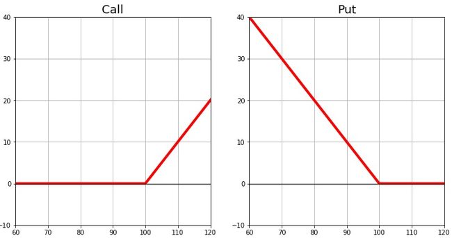
• Figure: 一个子图的例子
  (注释：这里，可以把Figure，即fig理解为一张大画布，你把它分成了两个子区域(sub1和sub2)，然后在每个子区域各画了一幅图。)

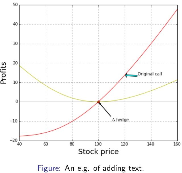
在绘制的图上添加文本和注释 (Adding texts to plots)

import numpy as np
from scipy.stats import norm
import matplotlib.pyplot as plt

def call(S, K=100, T=0.5, vol=0.6, r=0.05):
    d1 = (np.log(S/K) + (r + 0.5 * vol**2) \
          *T) / np.sqrt(T) / vol
    d2 = (np.log(S/K) + (r - 0.5 * vol**2) \
          *T) / np.sqrt(T) / vol
    return S * norm.cdf(d1) - K * \
    np.exp(-r * T) * norm.cdf(d2)

def delta(S, K=100, T=0.5, vol=0.6, r=0.05):
    d1 = (np.log(S/K) + (r + 0.5 * vol**2)\
          *T) / np.sqrt(T) / vol
    return norm.cdf(d1)

(Code continues:)

S = np.linspace(40, 161, 100)
fig = plt.figure(figsize=(7, 6))
ax = fig.add_subplot(111)
plt.plot(S,(call(S)-call(100)),’r’,lw=1)
plt.plot(100, 0, ’ro’, lw=1)
plt.plot(S,np.zeros_like(S), ’black’, lw = 1)
plt.plot(S,call(S)-delta(100)*S- \
    (call(100)-delta(100)*100), ’y’, lw = 1)

(Code continues:)

ax.annotate(’$\Delta$ hedge’, xy=(100, 0), \
            xytext=(110, -10),arrowprops= \
            dict(headwidth =3,width = 0.5, \
            facecolor=’black’, shrink=0.05))
ax.annotate(’Original call’, xy= \
            (120,call(120)-call(100)),xytext\
            =(130,call(120)-call(100)),\
            arrowprops=dict(headwidth =10,\
            width = 3, facecolor=’cyan’, \
            shrink=0.05))
plt.grid(True)
plt.xlim(40, 160)
plt.xlabel(’Stock price’, fontsize = 18)
plt.ylabel(’Profits’, fontsize = 18)

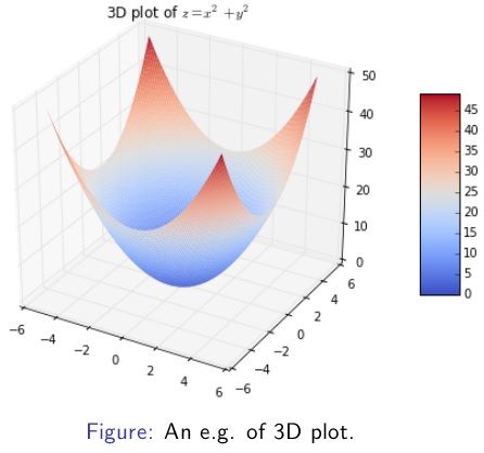
两个变量的函数3D制图（3D plot of a function with 2 variables）

import numpy as np
import matplotlib.pyplot as plt
from matplotlib import cm
from mpl_toolkits.mplot3d import Axes3D

x, y = np.mgrid[-5:5:100j, -5:5:100j]
z = x**2 + y**2
fig = plt.figure(figsize=(8, 6))
ax = plt.axes(projection='3d')
surf = ax.plot_surface(x, y, z, rstride=1,\
                       cmap=cm.coolwarm, cstride=1, \
                       linewidth=0)
fig.colorbar(surf, shrink=0.5, aspect=5)
plt.title('3D plot of $z = x^2 + y^2$')

3days_img016_3D_plot.jpg

实验3:atplotlib (Lab 3: Matplotlib)

• 用蓝线绘制以下函数 (Plot the following function with blue line)

  
  • 然后用红点标记坐标（1,2） (Then mark the coordinate (1, 2) with a red point.)

• 使用np.linspace()使t ∈ [0，2π]。 然后给 (Use np.linspace0 to make t ∈ [0，2π]. Then give)

• 针对X绘Y。 在这个情节中添加一个称为“Heart”的标题。 (Plot y against x. Add a title to this plot which is called "Heart" .)

• 针对x∈[-10,10], y∈[-10,10], 绘制3D函数 (Plot the 3D function for x∈[-10,10], y∈[-10,10])

  

---

Sympy

符号计算 (Symbolic computation)

• 到目前为止，我们只考虑了数值计算。 (So far, we only considered the numerical computation.)

• Python也可以通过模块表征进行符号计算。(Python can also work with symbolic computation via module sympy.)

• 符号计算可用于计算方程，积分等的显式解。 (Symbolic computation can be useful for calculating explicit solutions to equations, integrations and so on.)

声明一个符号变量 (Declare a symbol variable)

import sympy as sy

#声明x，y为变量
x = sy.Symbol('x')
y = sy.Symbol('y')
a, b = sy.symbols('a b')

#创建一个新符号（不是函数
f = x**2 + 2 - 2*x + x**2 -1
print(f)
#自动简化
g = x**2 + 2 - 2*x + x**2 -1
print(g)

符号的使用1：求解方程 (Use of symbol 1: Solve equations)

import sympy as sy

x  = sy.Symbol ('x')
y  = sy.Symbol('y')

# 给定[-1,1]  (give [-1, 1])
print(sy.solve (x**2 - 1))

# 不能证解决 (no guarantee for solution)
print(sy.solve(x**3  +  0.5*x**2 - 1))

# 用x的表达式表示y     (exepress x in terms of y)
print (sy.solve(x**3  +  y**2))

# 错误：找不到算法 (error:  no  algorithm  can  be  found)
print(sy.solve(x**x + 2*x - 1))

符号的使用2：集成 (Use of symbol 2: Integration)

import sympy as sy

x = sy.Symbol('x')
y = sy.Symbol( 'y')
b = sy.symbols ( 'a b')

# 单变量 single  variable
f = sy.sin(x) + sy.exp(x)
print(sy.integrate(f, (x,  a,  b)))
print(sy.integrate(f, (x,  1,  2)))
print(sy.integrate(f, (x,  1.0,2.0)))
# 多变量 multi variables
g = sy.exp(x) + x * sy.sin(y)
print(sy.integrate(g, (y,a,b)))

符号的使用3：分化 (Use of symbol 3: Differentiation)

import sympy as sy
x =  sy.Symbol( 'x')
y =  sy.Symbol( 'y')
# 单变量 (single variable)
f = sy.cos(x) + x**x
print(sy . diff (f ,  x))
#  多变量  (multi variables)
g = sy.cos(y) * x + sy.log(y)
print(sy.diff (g,  y))

第二天结束，辛苦了

（传送门--去第三天）
（传送门--回第一天）