本文通过经典数据集MINST(手写0~9图片集),介绍二元分类的主要流程、预测指标,以及不同模型分类效果对比。
数据处理
1.获取和查看数据
%matplotlib inline
import matplotlib
import matplotlib.pyplot as plt
from sklearn.datasets import fetch_mldata
#获取本地数据集
mnist = fetch_mldata('MNIST original')
X,y = mnist['data'],mnist['target']
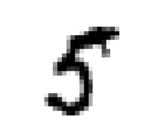
#展示单个数据
some_digit = X[]
some_digit_image = some_digit.reshape(28, 28)
plt.imshow(some_digit_image, cmap = matplotlib.cm.binary, interpolation='nearest')
plt.axis('off')
plt.show()
2.切分数据集
#随机打乱训练集
X_train, X_test, y_train, y_test = X[:60000],X[60000:],y[:60000],y[60000:]
import numpy as np
shuffle_index = np.random.permutation(60000)
X_train,y_train = X_train[shuffle_index], y_train[shuffle_index]
训练二元分类器
3.训练模型
数据集二元转化:数据集中,y值是包含0到9的数字,如果要做二元分类,那可以考虑只标记一个数字,比如5和非5,这就把0-9的数据集变成了bool的数据集。
模型选择:这里用的是随机梯度下降算法(SGD)。
# 转换数据集
y_train_5 = (y_train==5)
y_test_5 = (y_test==5)
# 训练模型
from sklearn.linear_model import SGDClassifier
sgd_clf = SGDClassifier(random_state=77)
sgd_clf.fit(X_train, y_train_5)
4.交叉验证
两种方式:
cross_val_score获取K折数据得分值;
cross_val_predict获取K折的预测数据。
虽然以下的数据显示中,K折的得分看似很高(0.95左右),但并不能代表预测的足够好了,因为原始数据中5的比例只占10%,只要预测非5,都可以达到0.9,所以我们要有其它更精确的预测指标。
from sklearn.model_selection import cross_val_score
from sklearn.model_selection import cross_val_predict
y_train_scores = cross_val_score(sgd_clf, X_train, y_train_5, cv=3, scoring='accuracy')
# array([0.9544, 0.9465, 0.9629])
y_train_pred = cross_val_predict(sgd_clf, X_train, y_train_5, cv=3)
# array([[54266,   313],
#       [ 2411,  3010]])
预测指标
5.精度和召回率
TN:真负类, FP:假正类
FN:假负类, TP:真正类
,
from sklearn.metrics import precision_score, recall_score
precision_score(y_train_5, y_train_pred) #精度
recall_score(y_train_5,y_train_pred) #召回率
6.分数
- 我们需要把精度和召回率组合成一个单一的指标,成为分数。精度和召回率较相近,分值较高。
7.精度/召回权衡
我们不能同时增加精度并较少召回率,反之亦然。这时我们需要精度/召回率权衡。
以SGDClassifier(随机梯度下降分类器)为例,它是如何进行分类决策的呢?
对于每个实例,它会基于决策函数计算出一个分值,如果该值大于阈值,则判为正类,否则为负类。 可以用decision_function()方法返回实例的分值。
那我们要如何决定使用什么阈值呢?
首先,我们获取训练集中所有实例的分数,然后利用分数来计算所有可能的阈值的精度和召回率,用图像绘制出精度和召回率相对于阈值的函数图,这样就可以通过轻松选择阈值来实现最佳的精度/召回率权衡了。 这条曲线也被成为PR曲线。
代码如下:
from sklearn.metrics import precision_recall_curve
# 获取y得分
y_scores = cross_val_predict(sgd_clf, X_train, y_train_5, cv=3, method='decision_function')
# 获取精确率、召回率、阈值
precisions, recalls, thresholds = precision_recall_curve(y_train_5, y_scores)

def plot_precision_recall_vs_threshold(precisions, recalls, thresholds):
    plt.plot(thresholds, precisions[:-1], "b--", label='Precision')
    plt.plot(thresholds, recalls[:-1], "g-", label="Recall")
    plt.xlabel("Threshold")
    plt.legend(loc="upper left")
    plt.ylim([0,1])
plot_precision_recall_vs_threshold(precisions, recalls, thresholds)
plt.show()

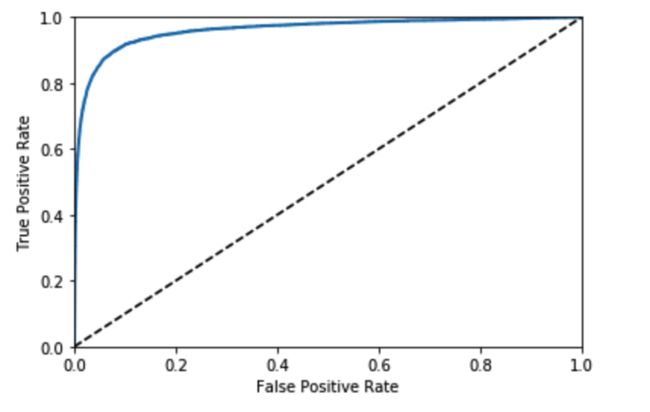
8.ROC曲线
ROC曲线绘制的是真正类率(召回率/tpr)和假正类率(fpr)的关系。可用曲线的面积(AUC分数)来代表曲线的效果。代码与绘制如下。
from sklearn.metrics import roc_curve,roc_auc_score
fpr, tpr, thresholds = roc_curve(y_train_5, y_scores)
def plot_roc_curve(fpr, tpr, label=None):
    plt.plot(fpr, tpr, linewidth=2, label=label)
    plt.plot([0,1],[0,1],'k--')
    plt.axis([0,1,0,1])
    plt.xlabel('False Positive Rate')
    plt.ylabel('True Positive Rate')
plot_roc_curve(fpr, tpr)
plt.show()

roc_auc_score(y_train_5, y_scores)
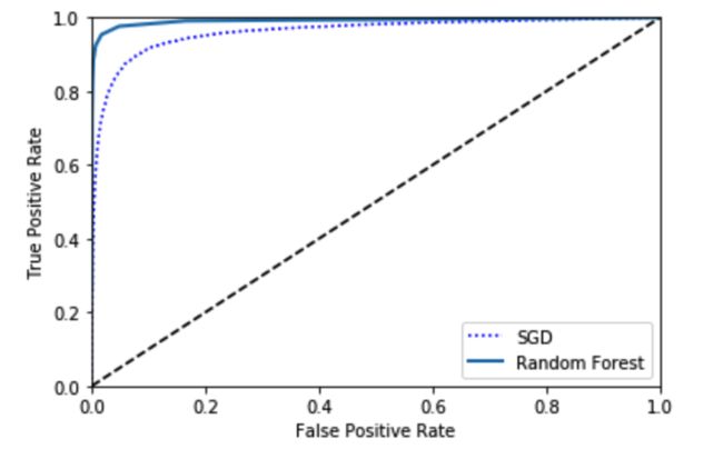
9.对比不同模型效果
在对比不同模型的分类效果时,可同时绘制ROC曲线来看看。以下是随机森林分类器,和SGD分类器的对比。
# 注:RandomForestClassifier没有decision_function()函数,用predict_proba代替。

from sklearn.ensemble import RandomForestClassifier

forest_clf = RandomForestClassifier(random_state=77)
y_probas_forest = cross_val_predict(forest_clf, X_train, y_train_5, cv=3, method='predict_proba')
y_scores_forest = y_probas_forest[:,1]
fpr_forest,tpr_forest,thresholds_forest = roc_curve(y_train_5,y_scores_forest)
plt.plot(fpr, tpr, 'b:', label='SGD')
plot_roc_curve(fpr_forest, tpr_forest, 'Random Forest')
plt.legend(loc='lower right')
plt.show()
roc_auc_score(y_train_5, y_scores_forest)
总结
二元分类的问题,要比较不同模型的效果,关键在于指标的理解和运用,要多多练习。