Computational Physics Homework 9 of Mobingbizhen

1.Abstract

• EXERCISES

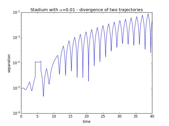
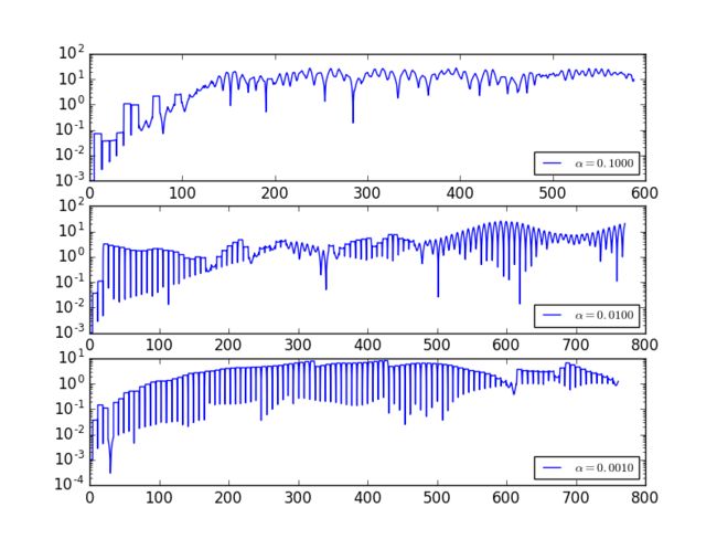
3.30. Investigate the Lyapunov exponent of the stadium billiard for several values of α. You can do this qualitatively by examining the behavior for only one set of initial conditions for each value of α you consider, or more quantitatively by averaging over a range of initial conditions for each value of α.

---

---

2.Background

• Lorenz Model

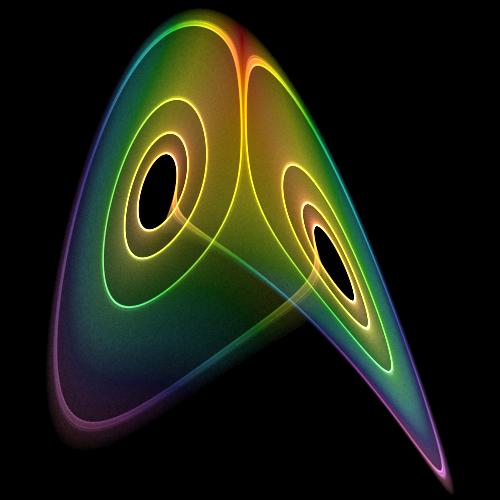
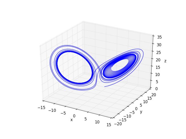
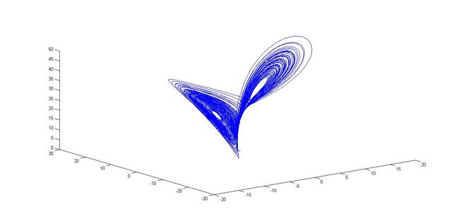
The Lorenz system is a system of ordinary differential equations(the Lorenz equations, note it is not Lorentz) first studied by Edward Lorenz. It is notable for having chaotic solutions for certain parameter values and initial conditions. In particular, the Lorenz attractor is a set of chaotic solutions of the Lorenz system which, when plotted, resemble a butterfly or figure eight.

A Trajectory Through Phase Space in a Lorenz Attractor

Intermittent Lorenz attractor - Chaoscope

• Butterfly Effect (in physical systems)

in weather

The butterfly effect is most familiar in terms of weather; it can easily be demonstrated in standard weather prediction models, for example. The climate scientists James Annan and William Connolley explain that chaos is important in the development of weather prediction methods; models are sensitive to initial conditions. They add the caveat: "Of course the existence of an unknown butterfly flapping its wings has no direct bearing on weather forecasts, since it will take far too long for such a small perturbation to grow to a significant size, and we have many more immediate uncertainties to worry about. So the direct impact of this phenomenon on weather prediction is often somewhat overstated."

in quantum mechanics

The potential for sensitive dependence on initial conditions (the butterfly effect) has been studied in a number of cases in semiclassical and quantum physics including atoms in strong fields and the anisotropic Kepler problem. Some authors have argued that extreme (exponential) dependence on initial conditions is not expected in pure quantum treatments; however, the sensitive dependence on initial conditions demonstrated in classical motion is included in the semiclassical treatments developed by Martin Gutzwiller and Delos and co-workers.
Other authors suggest that the butterfly effect can be observed in quantum systems. Karkuszewski et al. consider the time evolution of quantum systems which have slightly different Hamiltonians. They investigate the level of sensitivity of quantum systems to small changes in their given Hamiltonians. Poulin et al. presented a quantum algorithm to measure fidelity decay, which "measures the rate at which identical initial states diverge when subjected to slightly different dynamics". They consider fidelity decay to be "the closest quantum analog to the (purely classical) butterfly effect". Whereas the classical butterfly effect considers the effect of a small change in the position and/or velocity of an object in a given Hamiltonian system, the quantum butterfly effect considers the effect of a small change in the Hamiltonian system with a given initial position and velocity. This quantum butterfly effect has been demonstrated experimentally. Quantum and semiclassical treatments of system sensitivity to initial conditions are known as quantum chaos.

• 3D plotting (Python & VPython & Matlab)

Here comes the show：

(Code)

**Python** simulation of the Lorenz model

**Matlab** simulation of the Lorenz model

**VPython** simulation of the billiard problem

---

---

3.Main

• (As usual,In SI, angles in radians)

• Formulation

Except for the collisions with the walls, the motion of the billiard is quite simple. Between collisions the velocity is constant so we have

where vx and vy change only through collisions with the walls.

After locating the collision point, we need to do a little vector manipulation. The initial velocity vector vi = (vx, vy) is already known, since vx and vy are known. We must next obtain the unit vector normal to the wall at the point of collision, n. It is then useful to calculate the components of vi parallel to the wall. These are just

Once we have the components of vi we can reflect the billiard. A mirrorlike reflection reverses the perpendicular component of velocity, but leaves the parallel component unchanged. Hence, the velocity after reflection from the wall is

• Algorithm

Nothing to emphasize

• Thinking

After each time step we must check to see if there has been a collision with one of the walls, that is, if the newly calculated position puts the billiard off the table. When this happens the program must backtrack to locate the position where the collision occurred. There are several ways to do this.
One way is to back the billiard up to the position at the previous time step and then use a much smaller time step [for example, a factor of 100 smaller than the time step used to initially integrate (3.30)], so as to move the billiard in much smaller steps. When the billiard then goes off the table (again), we take the location after that iteration to be the point of collision.

• Results

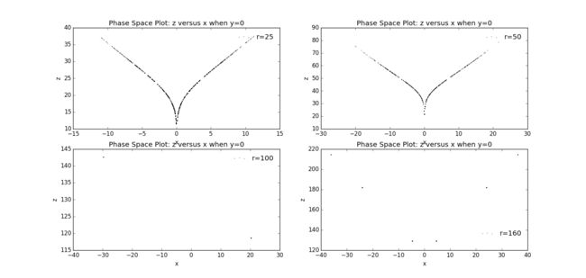
1. Firstly, I will show some of the figures that have emerged in Section 3.6 as a review.

2. Then, I will focus on section 3.7 - THE BILLIARD PROBLEM.

Review :

** r=25, σ=10, b=8/3, dt=0.0001s, time=50s**

Phase plot projected onto xOy, xOz, yOz plain

Attractors when x=0 (left) and y=0 (right)

Phase plot projected onto xOz plain

Attractors when x=0 with various r values

Attractors when y=0 with various r values

Then I am getting down to business:

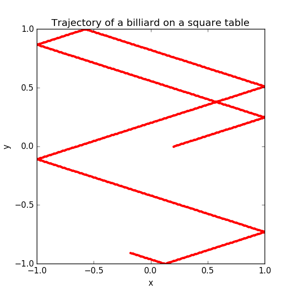
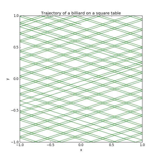
■ Square boundary

Let's show this in a more elegant way

or simpler

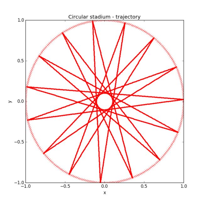
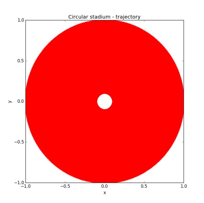
** Circular boundary**

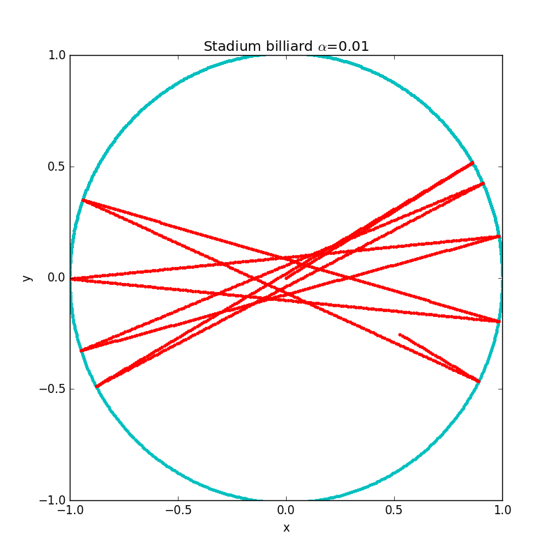
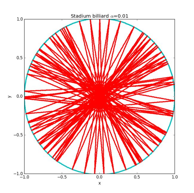
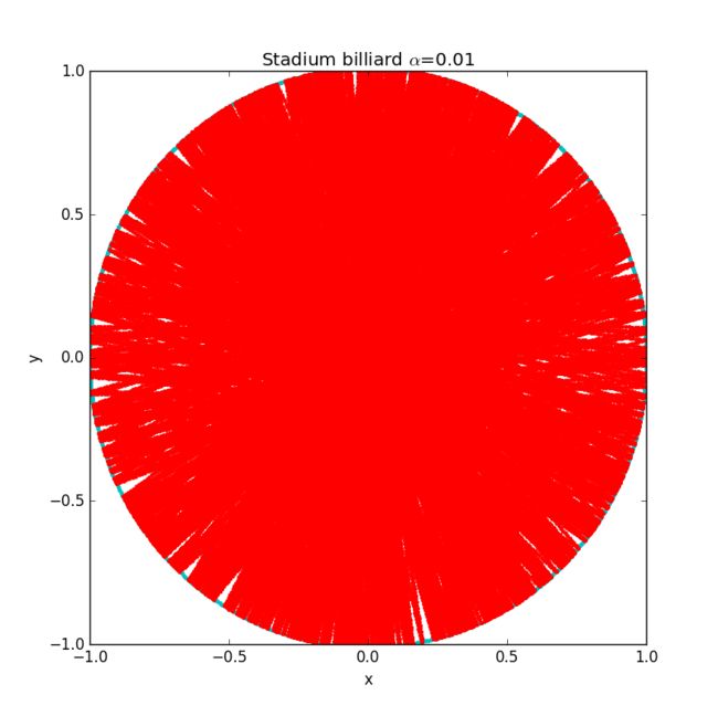
** Stadium boundary **

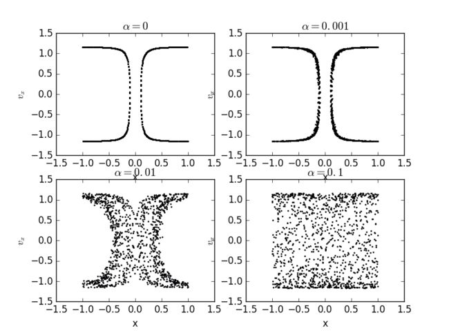
　 α = 0.01

**░ Phase space **

☰ Trajectory divergence

---

---

4.Conclusion

Ths chaotic system will present when the boundary is composed by some shapes (different or same). If the boundary is a simple regular shape, the chaotic situation cannot be observed.

---

---

5.Acknowledgement

• Prof. Cai
• Wikipedia
• Wang Shixing
• Chen Feng
• Tan Mingjun (Tan Shan)
• ZZT (Zhang Zitong)