利用matlab编写实现显示fmri切片slice图像 混合显示 不同侧面显示 可叠加t检验图显示 by DR. Rajeev Raizada

1.参考 reference

 

　　1. tutorial主页：http://www.bcs.rochester.edu/people/raizada/fmri-matlab.htm。

　　2.speech_brain_images.mat数据：speech_brain_images.mat。

　　3.showing_brain_images_tutorial显示大脑图像代码：showing_brain_images_tutorial.m 。

　　4.overlaying_Tmaps_tutorial.m叠加t检验统计图：overlaying_Tmaps_tutorial.m。

 

2.程序执行过程 run step by step

 

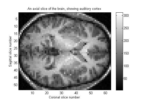
2.1 显示大脑axial 轴位 第18个切片的图像，以灰度图的方式显示

clear all;
close all; 

load speech_brain_images.mat

whos

%%%% This is the output that you should get:
%
% Name Size Bytes Class
%
% speech_Tmap 53x63x46 1228752 double array
% subj_3danat 53x63x46 1228752 double array

 

%%%% Let's look at the 18th axial slice.
%%%% This goes through Heschl's gyrus, which is auditory cortex

 

axial_slice_number = 18;

axial_slice_vals = subj_3danat(:,:,axial_slice_number);

%%%% Let's look at this matrix in a figure

figure(1); 
clf; 

imagesc(axial_slice_vals);

colormap gray; %%% Show the image in grayscale.

colorbar; %%% Put up a colorbar on the right, 

axis('image'); %%%% Lock the image to have the same proportions

title('An axial slice of the brain, showing auditory cortex');

xlabel('Coronal slice number');
ylabel('Sagittal slice number');

结果：

　　

 

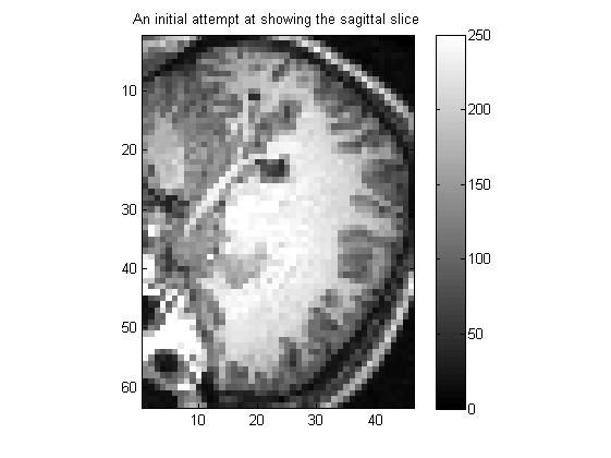
2.2 显示大脑sagittal矢状面 第20个切片的图像，以灰度图的方式显示

sagittal_slice_number = 20;

sagittal_slice_vals = subj_3danat(sagittal_slice_number,:,:);

%%%% Let's look at the variables in our workspace again

whos

%%%% Note that even though sagittal_slice_vals is just one slice,
% sagittal_slice_vals 1x63x46 23184 double array
%
% It turns out that the Matlab image command won't accept 3D matrices,
% so we need to get rid of this redundant one-voxel-wide dimension.
% Luckily, Matlab has a function that does precisely this, called squeeze.

sagittal_slice_2D = squeeze(sagittal_slice_vals);

%%% Get rid of the redundant 3rd dimension

%%%% Let's look at all the variables in our workspace
%%%% that start with "sagit"

whos sagit*

%%%% Squeeze worked! It made our sagittal slice 2D instead of 3D
%
% sagittal_slice_2D 63x46 23184 double array

%%%% Now we can plot it

figure(2); 

clf; 

imagesc(sagittal_slice_2D);

colormap gray; %%% Make it a grayscale plot

colorbar; %%% Show how the image intensities map onto the colormap
axis('image'); %%% Make the proportions correct
title('An initial attempt at showing the sagittal slice');

 

结果：

　

 

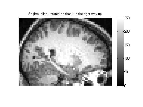
2.3 将上面大脑矢状面 图像旋转90度，以正常方式显示

caxis([ 0 250 ]); % Keep the black value at 0, but set the white value to 250

%%%% That makes the image look a lot better!
%%%% Now let's redraw the colorbar to see what the new colour-scaling is.

colorbar;

 

rotated_sagittal_slice = rot90(sagittal_slice_2D);

figure(3); %%% Make a new figure window, Fig.3
clf; %%% Clear the figure

imagesc(rotated_sagittal_slice);
%%% Show the image, with the brightness scaled
%%% so that the darkest is black and lightest is white

colormap gray; %%% Make it a grayscale plot
caxis([ 0 250 ]); % Keep the black value at 0, but set the white value to 250
colorbar; %%% Show how the image intensities map onto the colormap
axis('image'); %%% Make the proportions correct

title('Sagittal slice, rotated so that it is the right way up');

%%% For showing images, we often don't want to see the numbers
%%% on the x-axis and y-axis. We can turn these off using this command:

axis('off'); %%% Turn off the numbers running along the axes

结果：

　

 

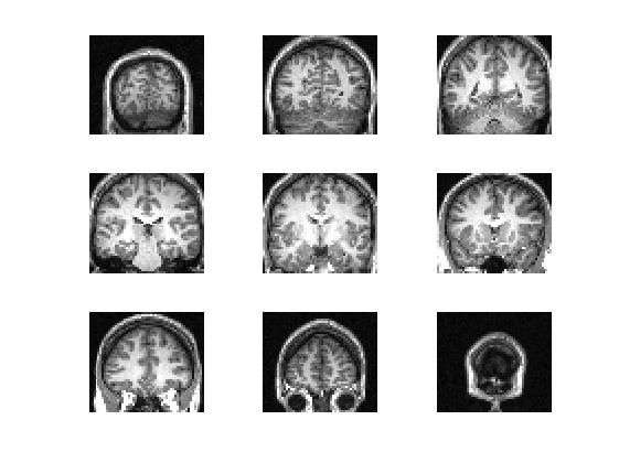
2.4 利用subplot()按灰度图显示大脑冠状面9个切片的图像

figure(4); %%% Make a new figure, Fig.4
clf; %%% Clear the figure

for loop_counter = 1:9, %%% Go around 9 times, adding one to the
%%% value of loop_counter each time.

coronal_slice_number = 7*loop_counter;
%%% Loop counter goes 1,2,3,...,9
%%% so this gives slices 7,14,21,...,63

coronal_slice_vals = subj_3danat(:,coronal_slice_number,:);
%%% The coronal slice is the 2nd dimension.
%%% So, read out that slice from the 3D subj_3danat matrix
%%% The ":" signs in the 1st and 3rd coordinate positions
%%% mean "give me all the x-vals and all the z-vals in that slice"

coronal_slice_2D = squeeze(coronal_slice_vals);
%%% We have to use squeeze to take out the redundant
%%% one-voxel-wide 2nd dimension, since imagesc will
%%% not let us display a 3D matrix

rotated_coronal_slice = rot90(coronal_slice_2D);
%%% Roate the slice by 90 degrees, to make it the right way up

subplot(3,3,loop_counter);
%%% Make a 3x3 array of subplots,
%%% and draw into the "loop_counter"-th one

imagesc(rotated_coronal_slice); %%% Make the image
colormap gray; %%% Make it grayscale

caxis([ 0 250 ]);
%%% So that very intense voxels don't make everything
%%% else look dark, set the black-value to 0,
%%% and set the white value to 250, like we did above.

axis('image'); %%% Make the proportions of the image correct

axis('off'); %%% Turn off the numbers on the x- and y-axes

end; %%% The end of this for-loop
%%% If loop_counter is less than 9, then add 1 to it,
%%% and then go back to the beginning.
%%% If loop_counter is 9, then stop --- the looping is finished.

结果：

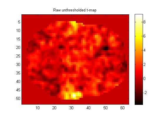
2.5 显示大脑axial 轴位 第18个切片的图像，不过以hot图的方式显示

axial_slice_number = 18;

%%%% The matrix containing a brain-full of voxels
%%%% with t-statistic numbers in them is called speech_Tmap

axial_slice_Tmap_vals = speech_Tmap(:,:,axial_slice_number);

%%%% Squeeze it, to get rid of the nuisance one-voxel wide 3rd dimension
%%%% in case there is one. (There might not always be, depending on
%%%% what type of slice you are taking. But it's a good idea to squeeze
%%%% all the time anyway, because it will make your programs more robust).

axial_slice_Tmap_2D = squeeze(axial_slice_Tmap_vals);

%%%% Now let's show this matrix as an image, in the way we did above.

figure(5);
clf;
imagesc(axial_slice_Tmap_2D);
axis('image'); %%% Make the proportions of the image correct
title('Raw unthresholded t-map');

%%%% For functional maps, a nice colormap to use is called "hot"
%%%% This makes the lowest numbers black, and then the colours
%%%% get "warmer" as the numbers increase: red, orange, yellow, white
%%%% To see a number of useful colormaps, type
%%%% help graph3d
%%%% into the Matlab command window.

colormap hot;

%%% Let's make a colorbar to show us which t-map values get shown
%%% as which colours.
colorbar;

结果：

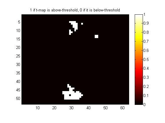
2.6 设定一个阈值，如果矩阵中有元素大于Tmap_threshold ，就设为1，否则置为0。

Tmap_threshold = 3.5;

%%%% In Matlab, the way to figure out which voxels have values
%%%% above this threshold is to make a matrix that has a 1 in every
%%%% above-threshold voxel, and a zero everywhere else.
%%%%
%%%% In other words, we want a 1 in every voxel where the statement
%%%% "this voxel's intensity is greater than the threshold" is true.
%%%%
%%%% Here's how we do that in Matlab:

True_or_false_map = ( axial_slice_Tmap_2D > Tmap_threshold );

%%%% The matrix will have a 1 in it in every voxel where the
%%%% bracketed expression ( axial_slice_Tmap_2D > Tmap_threshold )
%%%% is true, i.e. in all the above-threshold voxels,
%%%% and a zero in all the voxels where it's false.
%%%% Making true-or-false matrices like this turns out
%%%% to be useful in all kinds of circumstances.

%%%% Let's have a look at our True_or_false_map:

figure(6);
clf;
imagesc(True_or_false_map);
axis('image');
colormap hot;
colorbar;
title('1 if t-map is above-threshold, 0 if it is below-threshold');

结果：

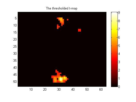
2.7 将阈值图矩阵和真实的图像做“点乘运算”，过滤非激活元素

Above_threshold_Tmap = True_or_false_map .* axial_slice_Tmap_2D;

%%%% Let's look at our above-treshold T-map

figure(7);
clf;
imagesc(Above_threshold_Tmap);
axis('image');
colormap hot;
colorbar;
title('The thresholded t-map');

结果：

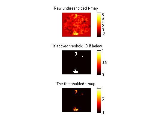
2.8 集中对比显示，阈值化前后的效果

figure(8);
clf;

subplot(3,1,1); %%% Three rows of subplots, one column, draw in the first one
imagesc(axial_slice_Tmap_2D);
axis('image');
axis('off');
colormap hot;
colorbar;
title('Raw unthresholded t-map');

subplot(3,1,2); %%% The last argument is 2, meaning
%%% "Draw in the 2nd of the three subplots"
imagesc(True_or_false_map);
axis('image');
axis('off');
colormap hot;
colorbar;
title('1 if above-threshold, 0 if below');

subplot(3,1,3); %%% The last argument is 3, meaning
%%% "Draw in the 3rd of the three subplots"
imagesc(Above_threshold_Tmap);
axis('image');
axis('off');
colormap hot;
colorbar;
title('The thresholded t-map');

 

结果：

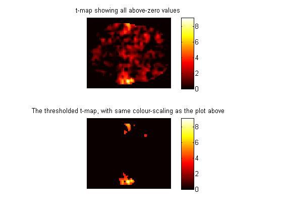
2.9 再做一下对比，对没有叠加阈值图的大脑图像，做对比对拉伸。然后，查看效果：就是激活区域，仍然是最亮的。

max_Tmap_value = max(max(axial_slice_Tmap_2D)); % Single biggest t-map score

%%%% Recall that the argument that we give to caxis is a two-element
%%%% vector, containing the maximum and minimum values we want
%%%% for the colorbar.

colorbar_min_and_max_vals = [ 0 max_Tmap_value ];

%%%% Now we can plot our thresholded and unthresholded t-maps
%%%% side-by-side, using exactly the same colour scaling in both.

figure(9);
clf;

subplot(2,1,1); %%% Two rows of subplots, one column, draw in the first one
imagesc(axial_slice_Tmap_2D);
axis('image');
axis('off');
colormap hot;

%%% Now set the colour scaling to what we want.
%%% Do this before making the colorbar
caxis(colorbar_min_and_max_vals);

colorbar;
title('t-map showing all above-zero values');

subplot(2,1,2); %%% The last argument is 2, meaning
%%% "Draw in the 2nd of the two subplots"
imagesc(Above_threshold_Tmap);
axis('image');
axis('off');
colormap hot;
caxis(colorbar_min_and_max_vals);
%%% This subplot will now have the same colour scaling as the first one
colorbar;
title('The thresholded t-map, with same colour-scaling as the plot above');

结果：

2.10 在spm中，可以通过滚动鼠标滚轮的方式，动态查看（按animation或者movie的方式）查看多层图像。

这里通过键盘按键的方式，进行了实现。不过，智能实现一次循环。

figure(10); 
clf; 

set(gcf,'doublebuffer','on'); 

for sagittal_slice_number = 1:53, 

%%% There are 53 sagittal slices, and this loop
%%% goes around 53 times, adding one to the
%%% value of sagittal_slice_number each time.

sagittal_slice_vals = subj_3danat(sagittal_slice_number,:,:);

sagittal_slice_2D = squeeze(sagittal_slice_vals);

rotated_sagittal_slice = rot90(sagittal_slice_2D);


imagesc(rotated_sagittal_slice); 
colormap gray; 

caxis([ 0 250 ]);

axis('image');

xlabel(['Sagittal slice number ' num2str(sagittal_slice_number) ]);

title('Press any key to show the next slice');

pause; 
%%% After the key press, the program continues,

end; %%% The end of this for-loop

结果：

  

 

 

the end 完整代码

 

%%%% Tutorial on how to show brain images in Matlab

%%%% Written by Rajeev Raizada, July 23, 2002.

%%%% 

%%%% To run it, you need the file containing the brain images:

%%%% speech_brain_images.mat (2.3Mb)

%%%% Probably the best way to look at this program is to read through it

%%%% line by line, and paste each line into the Matlab command window

%%%% in turn. That way, you can see what effect each individual command has.

%%%%

%%%% Anything with a % sign in front of it is a comment.

%%%% These will probably show up red in your Matlab Editor.

%%%% Everything else is a Matlab command, that you can copy and

%%%% paste into the Matlab command window.

%%%%

%%%% Alternatively, you can run the program directly by typing 

%%%%

%%%%   showing_brain_images_tutorial

%%%%

%%%% into your Matlab command window. 

%%%% Do not type ".m" at the end.

%%%% If you run the program all at once, all the Figure windows

%%%% will get made at once and will be sitting on top of each other.

%%%% You can move them around to see the ones that are hidden beneath.

%%%%

%%%% Please mail any comments or suggestions to: [email protected]



%%%%%%% First, clear the Matlab workspace of any variables

%%%%%%% that it might have stored in it, and close any existing figures



clear all;    %%% Empty the workspace of all variables

close all;    %%% Close any figures that might be open



%%%%%%% Load in the file containing the brain images

load speech_brain_images.mat



%%%%%%% Let's look at the variables that we've just loaded in

%%%%%%% The matlab command to do this is "whos"

%%%%%%% It shows what the variables are called, what size they are,

%%%%%%% how much memory they take up, and what data-types they are.



whos



%%%% This is the output that you should get:

%

%  Name              Size         Bytes  Class

%

%  speech_Tmap      53x63x46    1228752  double array

%  subj_3danat      53x63x46    1228752  double array

 

% This means that the variables "speech_Tmap" and "subj_3danat"

% are both 3-dimensional matrices.

% Each one has  53 rows, 63 columns, and 46 slices in the third dimension.



% Each matrix is a brain-full of voxel values.

% These particular images have already been preprocessed by SPM,

% which means that they have already been squashed and stretched

% in order to match onto a standard brain-template.

% This process of squashing and stretching is called spatial 

% normalisation. The advantage of normalising our images

% onto this standard space is that we can overlap one image 

% on top of another one, and they will line-up correctly.

% This is useful both for overlaying functional maps on top

% of anatomical images, and also for averaging together 

% functional maps from different subjects.

%

% There are a variety of different ways of doing spatial normalisation.

% The most common one is to squash and stretch the brain images

% to fit a standard brain that was mapped out by Talairach.

% That's called putting the brain into Talairach-space, or "Talairach-ing". 

% SPM uses MNI-space, which is  similar to Talairach space.

% Freesurfer/FS-FAST uses a different approach: the grey

% matter is segmented, inflated, and then normalised onto

% a spherical surface.

%

% The ordering of the dimensions in our images is as follows:

%

% The first dimension is the MRI x-direction: ear-to-ear

% x specifies the x-th sagittal slice, and as you

% increase x you move from one ear to the other ear.

% (Whether this means going from right-to-left or left-to-right

% depends on whether you are using neurological or radiological convention).

% Neurological convention: left-is-left.

% Radiological convention: left-is-right.

%

% The second dimension is the MRI y-direction: back-to-front

% y specifies the y-th coronal slice, and as you

% increase y you move from the back of the brain to the front.

%

% The third dimension is the MRI z-direction: feet-to-head

% z specifies the z-th axial slice, and as you

% increase y you move from the bottom of the brain to the top.





%%%% Let's look at the 18th axial slice.

%%%% This goes through Heschl's gyrus, which is auditory cortex



axial_slice_number = 18;



%%%% The axial slices are specified in the z-direction,

%%%% which means that we want to specify the third coordinate.

%%%% We want all the data in that given z-slice, 

%%%% i.e. the data for all the x-values and all the y-values

%%%% In Matlab, you say that you want all the values in

%%%% a particular dimension by putting a colon sign there.



%%%% Let's extract the data from the anatomical brain image,

%%%% which is stored in the matrix called subj_3danat



%%%% So, to extract the particular axial slice that we want,

%%%% and to get all the x-values and y-values in that slice,

%%%% we do this:



axial_slice_vals = subj_3danat(:,:,axial_slice_number);



%%%% Let's look at this matrix in a figure



figure(1);    %%% Open a new figure window, Figure 1

clf;          %%% Clear the figure



imagesc(axial_slice_vals);

        %%% Display the matrix as an image. 

        %%% The columns in the matrix get displayed in the x-direction

        %%% going from left to right, and the rows get displayed in

        %%% the y-direction, going from top to bottom.

        %%% Each pixel in the image shows the value of one entry

        %%% in the matrix. 

        

%%% The colour of each pixel is determined by the value of the

%%% entry in the matrix. Typically we want low numbers to give

%%% dark colours, and high numbers to give bright colours.

%%% Matlab has various built in colormaps that do this.

%%% For anatomical images, we typically want to view them in grayscale

%%% We achieve this with the following Matlab command



colormap gray;  %%% Show the image in grayscale.



%%%% The default colormap is called "jet". It goes from

%%%% dark blue, up through light blue, yellow and red.

%%%% That's probably how your brain picture looked before

%%%% you pasted the command "colormap gray" into the command window.



%%%% Note that the command we used to show the image was not

%%%% image(), it was imagesc(). Note the "sc" after image.

%%%% This means "image scaled". The scaling means that Matlab

%%%% automatically sets it so that the lowest number in the matrix

%%%% gets shown as the first colour in the colormap, which is black

%%%% in this case, and the highest number gets shown as the 

%%%% last colour in the colormap, which is white for colormap gray.

%%%% So, the darkest pixel is black and the lightest is white.



%%%% It would be nice to see how the numbers in the image

%%%% correspond to the colours in the colormap.

%%%% The Matlab command "colorbar" does this.



colorbar;   %%% Put up a colorbar on the right, 

            %%% showing how the numbers get mapped to colours





%%%% As it happens, the axial slice is more or less the same

%%%% shape as the default Matlab figure window. 

%%%% So, its proportions probably look about right.

%%%% But actually the proportions are just following the shape

%%%% of the figure window. Try grabbing a corner of the

%%%% figure window with the mouse and dragging to resize the window.

%%%% You'll see that the image gets stretched and squashed 

%%%% to follow the window size.



%%%% It would be good to lock the image's aspect ratio

%%%% so that it has the correct proportions.

%%%% That way the image won't be stretched or squashed.

%%%% The command axis('image') does this.

            

axis('image');  %%%% Lock the image to have the same proportions

                %%%% as the matrix that it is displaying

                

%%% Let's give our figure a title, and let's label the axes



title('An axial slice of the brain, showing auditory cortex');

xlabel('Coronal slice number');

ylabel('Sagittal slice number');



%%%% Now try stretching and squashing the figure window, and

%%%% you'll see that the image always keeps the correct proportions



%%%% Now let's try looking at a sagittal slice, e.g. slice 20



sagittal_slice_number = 20;



%%%% The sagittal slices are in the MRI x-direction, which

%%%% is the first coordinate.



%%%% So, we specify the first coordinate, and put a colon sign

%%%% in the 2nd and 3rd coordinates, meaning 

%%%% "give me all the y and z values for the slice with this given x-value".



sagittal_slice_vals = subj_3danat(sagittal_slice_number,:,:);



%%%% Let's look at the variables in our workspace again



whos



%%%% Note that even though sagittal_slice_vals is just one slice,

%%%% i.e. it is 2-dimensional, it is showing up in the workspace

%%%% as a 3D matrix that is 1x63x46

%%%%

%%%% I.e. Even though we have set the x-dimension to just a single

%%%% value, namely sagittal_slice, that dimension hasn't disappeared.

%%%% It's still there in the matrix, it's just one voxel wide.

%

%   sagittal_slice_vals       1x63x46      23184  double array

%

% It turns out that the Matlab image command won't accept 3D matrices,

% so we need to get rid of this redundant one-voxel-wide dimension.

% Luckily, Matlab has a function that does precisely this, called squeeze.



sagittal_slice_2D = squeeze(sagittal_slice_vals);

                        %%% Get rid of the redundant 3rd dimension

                                

%%%% Let's look at all the variables in our workspace

%%%% that start with "sagit"



whos sagit*



%%%% Squeeze worked! It made our sagittal slice 2D instead of 3D

%

%  sagittal_slice_2D        63x46         23184  double array



%%%% Now we can plot it



figure(2);      %%% Make a new figure window, Fig.2

clf;            %%% Clear the figure



imagesc(sagittal_slice_2D); 

                %%% Show the image, with the brightness scaled 

                %%% so that the darkest is black and lightest is white



colormap gray;  %%% Make it a grayscale plot

colorbar;       %%% Show how the image intensities map onto the colormap

axis('image');  %%% Make the proportions correct

title('An initial attempt at showing the sagittal slice');



%%%% When we look at Figure 2, we can see that it doesn't look quite right

%%%% Firstly, it's the wrong way round. The eye is looking downwards!

%%%% Secondly, it's very dark, except for one very bright point, which

%%%% is a blood vessel. What has happened is that this one very intense

%%%% point got set to white, and everything else got scaled accordingly,

%%%% meaning that everything else gets shown as a dull gray.

%%%% We want to change the scaling of our colormap so that these 

%%%% less intense points get shown brighter. 

%%%% If you look at the colorbar in Figure 2, you can see that

%%%% the current scaling is that black is near to zero, 

%%%% and white is around 700-ish.



%%%% Maybe if we set the white-point to be 250, things would look better.

%%%% We might "over-expose" the most intense voxels and push them all

%%%% into being uniform white, but we'll get better contrast in the

%%%% parts of the brain that we care about.



%%%% The command to change the colour-scaling in Matlab is "caxis".

%%%% We give it a two numbers, put into square brackets to make

%%%% them into two-entry vector. 

%%%% The first number is the intensity value to set to black.

%%%% The second number is the intensity value to set to white.



caxis([ 0 250 ]); % Keep the black value at 0, but set the white value to 250 



%%%% That makes the image look a lot better!

%%%% Now let's redraw the colorbar to see what the new colour-scaling is.



colorbar;   



%%% Notice that the colorbar goes from 0 to 250 now, instead of 0 to 700.



%%% That has fixed one problem, but the image is still the wrong way round.

%%% The eyes are still facing down.

%%% We want to rotate the image by 90 degrees.

%%% The way we do this in Matlab is to rotate the matrix by 90 degrees,

%%% and then redraw the newly rotated matrix.



%%% The Matlab command to rotate a matrix by 90 degrees is called "rot90".



rotated_sagittal_slice = rot90(sagittal_slice_2D);



figure(3);      %%% Make a new figure window, Fig.3

clf;            %%% Clear the figure



imagesc(rotated_sagittal_slice); 

                %%% Show the image, with the brightness scaled 

                %%% so that the darkest is black and lightest is white



colormap gray;  %%% Make it a grayscale plot

caxis([ 0 250 ]); % Keep the black value at 0, but set the white value to 250 

colorbar;       %%% Show how the image intensities map onto the colormap

axis('image');  %%% Make the proportions correct



title('Sagittal slice, rotated so that it is the right way up');



%%% For showing images, we often don't want to see the numbers

%%% on the x-axis and y-axis. We can turn these off using this command:



axis('off');    %%% Turn off the numbers running along the axes





%%%%%%%%%%%%%%%%%  Making subplots  %%%%%%%%%%%%%%%%%%



%%%% Another useful trick is to show more than one plot

%%%% in a single figure window. 

%%%% The command "subplot" does this.



%%%% Subplot gets called with three arguments: 

%%%% 1. How many rows of subfigures you want

%%%% 2. How many columns of subfigures you want

%%%% 3. Which subfigure to plot in. 

%%%%    The subfigures are numbered in turn row-by-row

 

%%%% Let's make a figure window showing a 3x3 array

%%%% array of subplots, each one showing a different coronal slice

%%%% The coronal slices are the y-coordinate, the 2nd dimension,

%%%% and there are 63 of them.

%%%% This uses all the techniques that we learned above.



%%%% We'll use a for-loop

%%%% If you're pasting these lines into the Matlab command window,

%%%% you need to copy and paste all the lines below at once.



figure(4);      %%% Make a new figure, Fig.4

clf;            %%% Clear the figure



for loop_counter = 1:9,     %%% Go around 9 times, adding one to the 

                            %%% value of loop_counter each time.



    coronal_slice_number = 7*loop_counter;

            %%% Loop counter goes 1,2,3,...,9

            %%% so this gives slices 7,14,21,...,63

    

    coronal_slice_vals = subj_3danat(:,coronal_slice_number,:);

            %%% The coronal slice is the 2nd dimension.

            %%% So, read out that slice from the 3D subj_3danat matrix

            %%% The ":" signs in the 1st and 3rd coordinate positions

            %%% mean "give me all the x-vals and all the z-vals in that slice"



    coronal_slice_2D = squeeze(coronal_slice_vals);

            %%% We have to use squeeze to take out the redundant

            %%% one-voxel-wide 2nd dimension, since imagesc will 

            %%% not let us display a 3D matrix



    rotated_coronal_slice = rot90(coronal_slice_2D);

            %%% Roate the slice by 90 degrees, to make it the right way up

    

    subplot(3,3,loop_counter);

            %%% Make a 3x3 array of subplots, 

            %%% and draw into the "loop_counter"-th one



    imagesc(rotated_coronal_slice); %%% Make the image

    colormap gray;                  %%% Make it grayscale

    

    caxis([ 0 250 ]); 

            %%% So that very intense voxels don't make everything

            %%% else look dark, set the black-value to 0, 

            %%% and set the white value to 250, like we did above.

    

    axis('image');  %%% Make the proportions of the image correct



    axis('off');    %%% Turn off the numbers on the x- and y-axes

    

end;    %%% The end of this for-loop

        %%% If loop_counter is less than 9, then add 1 to it,

        %%% and then go back to the beginning. 

        %%% If loop_counter is 9, then stop --- the looping is finished.



        

%%%%%%%%%%%%%%%%%%%%%%%%%%%%%%%%%%%%%%%%%%%%%%%%%%%%%%%%%%%%

%%%%

%%%% Ok, that's enough of the anatomical images.

%%%% Let's try looking at some functional maps.

%%%% A functional map is an image, just like an anatomical,

%%%% except that each voxel's intensity represents the statistical

%%%% significance of BOLD activiation at that point, rather than

%%%% showing what type of anatomical tissue is there.

%%%%

%%%% There are various types of statistical values that

%%%% can be used in functional maps: t-values, Z-values, p-values.

%%%% A common one to use is the t-value (this is exactly the same

%%%% number as in a regular t-test).

%%%% The bigger the t-value, the more statistically significant

%%%% is the neural activation at that part of the brain.

%%%% A brain-full of t-values is called a t-map.

%%%%

%%%% Eventually we'll want to overlay these t-maps on top of 

%%%% the anatomical images, but it turns out that this a little trickier.

%%%% An accompanying program  overlaying_Tmaps_tutorial.m  

%%%% shows how to do that. 

%%%% That program is not meant to be introductory, it assumes

%%%% that you have already worked through this one first.

%%%%

%%%% Let's look at the t-map in the same axial slice that we

%%%% looked at in the anatomical image in Figure 1.

%%%% It's the 18th axial slice.

%%%% This goes through Heschl's gyrus, which is auditory cortex



axial_slice_number = 18;



%%%% The matrix containing a brain-full of voxels 

%%%% with t-statistic numbers in them is called   speech_Tmap



axial_slice_Tmap_vals = speech_Tmap(:,:,axial_slice_number);



%%%% Squeeze it, to get rid of the nuisance one-voxel wide 3rd dimension

%%%% in case there is one. (There might not always be, depending on

%%%% what type of slice you are taking. But it's a good idea to squeeze

%%%% all the time anyway, because it will make your programs more robust).



axial_slice_Tmap_2D = squeeze(axial_slice_Tmap_vals);



%%%% Now let's show this matrix as an image, in the way we did above.



figure(5);

clf;

imagesc(axial_slice_Tmap_2D);

axis('image');      %%% Make the proportions of the image correct

title('Raw unthresholded t-map');



%%%% For functional maps, a nice colormap to use is called "hot"

%%%% This makes the lowest numbers black, and then the colours

%%%% get "warmer" as the numbers increase: red, orange, yellow, white

%%%% To see a number of useful colormaps, type 

%%%%     help graph3d 

%%%% into the Matlab command window.



colormap hot;



%%% Let's make a colorbar to show us which t-map values get shown

%%% as which colours.

colorbar;   



%%%%%%%%%%%% How to show a thresholded t-map %%%%%%%%

%

% You can see from Figure 5 that the strongest activity is in auditory

% cortex, bilaterally. That's what we'd expect, given that it's speech.

% For some unknown reason the right cortex is activated more than the left

% in this particular image.

% 

% Often we want to show a thresholded statistical map.

% To do this, we need to do two things:

%

% 1. Figure out which voxels exceed our threshold.

% 2. Make a map that shows these voxels' values, but it zero everywhere else.



%%%% First of all, we need to set a threshold



Tmap_threshold = 3.5;



%%%% In Matlab, the way to figure out which voxels have values 

%%%% above this threshold is to make a matrix that has a 1 in every

%%%% above-threshold voxel, and a zero everywhere else.

%%%%

%%%% In other words, we want a 1 in every voxel where the statement

%%%% "this voxel's intensity is greater than the threshold" is true.

%%%%

%%%% Here's how we do that in Matlab:



True_or_false_map = ( axial_slice_Tmap_2D > Tmap_threshold );



%%%% The matrix will have a 1 in it in every voxel where the

%%%% bracketed expression ( axial_slice_Tmap_2D > Tmap_threshold )

%%%% is true, i.e. in all the above-threshold voxels, 

%%%% and a zero in all the voxels where it's false.

%%%% Making true-or-false matrices like this turns out

%%%% to be useful in all kinds of circumstances.



%%%% Let's have a look at our True_or_false_map:



figure(6);

clf;

imagesc(True_or_false_map);

axis('image');

colormap hot;

colorbar;

title('1 if t-map is above-threshold, 0 if it is below-threshold');



%%%% Notice that everything is black and white, 

%%%% even though we are using the colormap hot.

%%%% That's because everything is either 0 or 1,

%%%% so we're not seeing any of the nice mid-value oranges and yellows.

%%%%

%%%% So, what we want is to combine the True_or_false_map

%%%% with the map of continuous-valued actual t-map numbers.

%%%%

%%%% The way to do this is to multiply the True_or_false_map

%%%% element-by-element with the actual t-map.

%%%% "Element-by-element" means that, say, the Row-3,Column-5 entry

%%%% in the True_or_false_map gets multiplied by the Row-3,Column-5 entry

%%%% in the actual t-map. 

%%%% Note that this is NOT the same as matrix multiplication!

%%%% Also, the two matrices must be exactly the same size as each other.

%%%%

%%%% In above-threshold voxels, the result of the multiplication will be:

%%%%

%%%%  1 * t-map-value  

%%%%

%%%%  ( It's multiplied by one because the 

%%%%    True_or_false_map is 1 here, because this voxel is above-threshold )

%%%%

%%%% In below-threshold voxels, the result of the multiplication will be:

%%%%

%%%%  0 * t-map-value    because these voxels are below threshold

%%%%

%%%% The way to do element-by-element multiplication in Matlab is

%%%% to put a dot in front of the * sign.

%%%% So, A*B means "A matrix-multiplied by B", 

%%%% and A.*B (note the dot) means "A element-by-element multiplied by B"



Above_threshold_Tmap  =  True_or_false_map .* axial_slice_Tmap_2D;



%%%% Let's look at our above-treshold T-map



figure(7);

clf;

imagesc(Above_threshold_Tmap);

axis('image');

colormap hot;

colorbar;

title('The thresholded t-map');





%%%% It's interesting to look at the three maps we made side by side.

%%%% We'll use the subplot command from above, with one column and three rows.



figure(8);

clf;



subplot(3,1,1); %%% Three rows of subplots, one column, draw in the first one

imagesc(axial_slice_Tmap_2D);

axis('image');

axis('off');

colormap hot;

colorbar;

title('Raw unthresholded t-map');





subplot(3,1,2); %%% The last argument is 2, meaning

                %%% "Draw in the 2nd of the three subplots"

imagesc(True_or_false_map);

axis('image');

axis('off');

colormap hot;

colorbar;

title('1 if above-threshold, 0 if below');



subplot(3,1,3); %%% The last argument is 3, meaning

                %%% "Draw in the 3rd of the three subplots"

imagesc(Above_threshold_Tmap);

axis('image');

axis('off');

colormap hot;

colorbar;

title('The thresholded t-map');





%%%%% If you look carefully at Figure 8, you'll notice that the colours

%%%%% in the above-threshold voxels in the uppermost plot are not

%%%%% exactly the same as the colours in the lowermost plot.

%%%%% That's because the colorbar scalings are slightly different.

%%%%%

%%%%% The top image, which is of the raw untresholded map, 

%%%%% has numbers less than -2 in it, and these are shown as black.

%%%%% Notice how the top colorbar goes from -2something to 8something.

%%%%%

%%%%% But the lowermost image, of the thresholded map, 

%%%%% doesn't have any numbers in it less than zero.

%%%%% But it still goes just as high, as you can see from the colobar.

%%%%% So, the oranges and yellows get spread out along the number-line

%%%%% a little differently.

%%%%%

%%%%% When you are presenting images side-by-side, it's often better

%%%%% to have the same colour-scaling for all of them. 

%%%%% Otherwise it can be misleading.

%%%%% We learned above how to specify a fixed colobar scaling

%%%%% by using the command "caxis". Let's do that for our side-by-side plots.

%%%%%

%%%%% A good setting for the colorbar scaling would be to have zero shown

%%%%% as black, and to have the maximum value in the map shown as white.

%%%%% Note that setting zero to be the black-point will look the same as

%%%%% if we had thresholded the t-map at zero, because we won't see

%%%%% any of the negative parts of the t-map any more.

%%%%%

%%%%% To find what the maximum value is, we can use the Matlab command "max".

%%%%% It turns out that if we apply "max" to a 2D-matrix, it gives us

%%%%% a row-vector of numbers giving the maximum value for each column.

%%%%% But we just want the maximum value in the whole matrix.

%%%%% So, we use max twice. That way, we get a single number that is

%%%%% the maximum in the entire matrix.



max_Tmap_value = max(max(axial_slice_Tmap_2D)); % Single biggest t-map score



%%%% Recall that the argument that we give to caxis is a two-element

%%%% vector, containing the maximum and minimum values we want 

%%%% for the colorbar. 



colorbar_min_and_max_vals = [  0  max_Tmap_value  ];  



%%%% Now we can plot our thresholded and unthresholded t-maps 

%%%% side-by-side, using exactly the same colour scaling in both.



figure(9);

clf;



subplot(2,1,1); %%% Two rows of subplots, one column, draw in the first one

imagesc(axial_slice_Tmap_2D);

axis('image');

axis('off');

colormap hot;



%%% Now set the colour scaling to what we want. 

%%% Do this before making the colorbar

caxis(colorbar_min_and_max_vals);   



colorbar;

title('t-map showing all above-zero values');





subplot(2,1,2); %%% The last argument is 2, meaning

                %%% "Draw in the 2nd of the two subplots"

imagesc(Above_threshold_Tmap);

axis('image');

axis('off');

colormap hot;

caxis(colorbar_min_and_max_vals); 

    %%% This subplot will now have the same colour scaling as the first one

colorbar;

title('The thresholded t-map, with same colour-scaling as the plot above');





%%%%%%%% Doing a "fly-through" of the slices %%%%%%%%%%%%

%

% To make an animation of a "fly through" the slices,

% we use a loop very similar to the one we used for making

% Figure 4, with its nine subplots of various slices.

% Except this time, instead of showing the different slices

% next to each other, we'll show them all in the same place

% but in quick sequence, giving the effect of a movie.



figure(10);     %%% Make a new figure

clf;            %%% Clear the figure



%%% It turns out that there's a nifty Matlab trick that allows us 

%%% to rapidly redraw new images, without the window flickering.

%%% The command below does this. Preventing the flicker makes

%%% the movie look a *lot* nicer.



set(gcf,'doublebuffer','on');   

    % gcf means "get current figure".

    % So, this means "set double-buffering to be on in the current figure".

    % Double-buffering means that Matlab draws the figure into a virtual

    % figure window in memory first, before copying it to the actual screen.

    % That's not really important, the main thing is that it stops flicker.



for sagittal_slice_number = 1:53,       

                %%% There are 53 sagittal slices, and this loop

                %%% goes around 53 times, adding one to the 

                %%% value of sagittal_slice_number each time.



    sagittal_slice_vals = subj_3danat(sagittal_slice_number,:,:);

            %%% The sagittal slice is the 1st dimension, the x-direction.

            %%% So, read out that slice from the 3D subj_3danat matrix

            %%% The ":" signs in the 2nd and 3rd coordinate positions

            %%% mean "give me all the y-vals and all the z-vals in that slice"



    sagittal_slice_2D = squeeze(sagittal_slice_vals);

            %%% We have to use squeeze to take out the redundant

            %%% one-voxel-wide 1st dimension, since imagesc will 

            %%% not let us display a 3D matrix



    rotated_sagittal_slice = rot90(sagittal_slice_2D);

            %%% Roate the slice by 90 degrees, to make it the right way up

    

    imagesc(rotated_sagittal_slice);    %%% Make the image

    colormap gray;                      %%% Make it grayscale

    

    caxis([ 0 250 ]); 

            %%% So that very intense voxels don't make everything

            %%% else look dark, set the black-value to 0, 

            %%% and set the white value to 250, like we did above.

    

    axis('image');  %%% Make the proportions of the image correct

    

    %%%% Let's show in the x-axis label which slice we're at.

    %%%% We can do this by making a compound string containing

    %%%% so text, and then the slice-number (which is a numeral),

    %%%% turned into a string. We have to change the number into

    %%%% a string because to a computer the number 5 is one more than 4,

    %%%% but the string "5" is an particular ASCII character.

    %%%% The Matlab command num2str does this for us.

    %%%% We put the whole compound string inside [ square brackets ]

    

    xlabel(['Sagittal slice number ' num2str(sagittal_slice_number) ]); 



    %%%%% Before going to the next slice, wait for the user to press a key

    title('Press any key to show the next slice');

    

    pause;      %%% This pause command waits for a key-press

                %%% After the key press, the program continues,

                %%% reaches the "end" command below, and that "end"

                %%% either takes us back to beginning of the loop,

                %%% to show the next slice, or stops at the last slice.

    

end;    %%% The end of this for-loop

        %%% If sagittal_slice_number is less than 53, then add 1 to it,

        %%% and then go back to the beginning. 

        %%% If sagittal_slice_number is 53, then stop.