学习模型评估和超参数调整的最佳实践
Code Repository: https://github.com/rasbt/python-machine-learning-book-2nd-edition
文章目录
- Learning Best Practices for Model Evaluation and Hyperparameter Tuning
- Streamlining workflows with pipelines
- Loading the Breast Cancer Wisconsin dataset
- Combining transformers and estimators in a pipeline
- Using k-fold cross validation to assess model performance
- The holdout method
- K-fold cross-validation
- Debugging algorithms with learning curves
- Diagnosing bias and variance problems with learning curves
- Addressing over- and underfitting with validation curves
- Fine-tuning machine learning models via grid search
- Tuning hyperparameters via grid search
- Algorithm selection with nested cross-validation
- Looking at different performance evaluation metrics
- Reading a confusion matrix
- Additional Note
- Optimizing the precision and recall of a classification model
- Plotting a receiver operating characteristic
- The scoring metrics for multiclass classification
- Dealing with class imbalance
- Summary
Learning Best Practices for Model Evaluation and Hyperparameter Tuning
Note that the optional watermark extension is a small IPython notebook plugin that I developed to make the code reproducible. You can just skip the following line(s).
%load_ext watermark
%watermark -a "Sebastian Raschka" -u -d -v -p numpy,pandas,matplotlib,sklearn
Sebastian Raschka
last updated: 2017-09-03

CPython 3.6.1
IPython 6.1.0

numpy 1.12.1
pandas 0.20.3
matplotlib 2.0.2
sklearn 0.19.0
The use of watermark is optional. You can install this IPython extension via “pip install watermark”. For more information, please see: https://github.com/rasbt/watermark.
from IPython.display import Image
%matplotlib inline
Streamlining workflows with pipelines
…
Loading the Breast Cancer Wisconsin dataset
import pandas as pd

df = pd.read_csv('https://archive.ics.uci.edu/ml/'
                 'machine-learning-databases'
                 '/breast-cancer-wisconsin/wdbc.data', header=None)

# if the Breast Cancer dataset is temporarily unavailable from the
# UCI machine learning repository, un-comment the following line
# of code to load the dataset from a local path:

# df_wine = pd.read_csv('wdbc.data', header=None)

df.head()
| 0 | 1 | 2 | 3 | 4 | 5 | 6 | 7 | 8 | 9 | ... | 22 | 23 | 24 | 25 | 26 | 27 | 28 | 29 | 30 | 31 | |
|---|---|---|---|---|---|---|---|---|---|---|---|---|---|---|---|---|---|---|---|---|---|
| 0 | 842302 | M | 17.99 | 10.38 | 122.80 | 1001.0 | 0.11840 | 0.27760 | 0.3001 | 0.14710 | ... | 25.38 | 17.33 | 184.60 | 2019.0 | 0.1622 | 0.6656 | 0.7119 | 0.2654 | 0.4601 | 0.11890 |
| 1 | 842517 | M | 20.57 | 17.77 | 132.90 | 1326.0 | 0.08474 | 0.07864 | 0.0869 | 0.07017 | ... | 24.99 | 23.41 | 158.80 | 1956.0 | 0.1238 | 0.1866 | 0.2416 | 0.1860 | 0.2750 | 0.08902 |
| 2 | 84300903 | M | 19.69 | 21.25 | 130.00 | 1203.0 | 0.10960 | 0.15990 | 0.1974 | 0.12790 | ... | 23.57 | 25.53 | 152.50 | 1709.0 | 0.1444 | 0.4245 | 0.4504 | 0.2430 | 0.3613 | 0.08758 |
| 3 | 84348301 | M | 11.42 | 20.38 | 77.58 | 386.1 | 0.14250 | 0.28390 | 0.2414 | 0.10520 | ... | 14.91 | 26.50 | 98.87 | 567.7 | 0.2098 | 0.8663 | 0.6869 | 0.2575 | 0.6638 | 0.17300 |
| 4 | 84358402 | M | 20.29 | 14.34 | 135.10 | 1297.0 | 0.10030 | 0.13280 | 0.1980 | 0.10430 | ... | 22.54 | 16.67 | 152.20 | 1575.0 | 0.1374 | 0.2050 | 0.4000 | 0.1625 | 0.2364 | 0.07678 |
5 rows × 32 columns
df.shape
(569, 32)
from sklearn.preprocessing import LabelEncoder

X = df.loc[:, 2:].values
y = df.loc[:, 1].values
le = LabelEncoder()
y = le.fit_transform(y)
le.classes_
array(['B', 'M'], dtype=object)
le.transform(['M', 'B'])
array([1, 0])
from sklearn.model_selection import train_test_split

X_train, X_test, y_train, y_test = \
    train_test_split(X, y,
                     test_size=0.20,
                     stratify=y,
                     random_state=1)
Combining transformers and estimators in a pipeline
from sklearn.preprocessing import StandardScaler
from sklearn.decomposition import PCA
from sklearn.linear_model import LogisticRegression
from sklearn.pipeline import make_pipeline

pipe_lr = make_pipeline(StandardScaler(),
                        PCA(n_components=2),
                        LogisticRegression(random_state=1))

pipe_lr.fit(X_train, y_train)
y_pred = pipe_lr.predict(X_test)
print('Test Accuracy: %.3f' % pipe_lr.score(X_test, y_test))
Test Accuracy: 0.956
Image(filename='images/06_01.png', width=500)

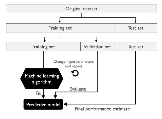
Using k-fold cross validation to assess model performance
…
The holdout method
Image(filename='images/06_02.png', width=500)
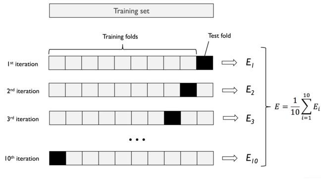
K-fold cross-validation
Image(filename='images/06_03.png', width=500)
import numpy as np
from sklearn.model_selection import StratifiedKFold


kfold = StratifiedKFold(n_splits=10,
                        random_state=1).split(X_train, y_train)

scores = []
for k, (train, test) in enumerate(kfold):
    pipe_lr.fit(X_train[train], y_train[train])
    score = pipe_lr.score(X_train[test], y_train[test])
    scores.append(score)
    print('Fold: %2d, Class dist.: %s, Acc: %.3f' % (k+1,
          np.bincount(y_train[train]), score))

print('\nCV accuracy: %.3f +/- %.3f' % (np.mean(scores), np.std(scores)))
Fold:  1, Class dist.: [256 153], Acc: 0.935
Fold:  2, Class dist.: [256 153], Acc: 0.935
Fold:  3, Class dist.: [256 153], Acc: 0.957
Fold:  4, Class dist.: [256 153], Acc: 0.957
Fold:  5, Class dist.: [256 153], Acc: 0.935
Fold:  6, Class dist.: [257 153], Acc: 0.956
Fold:  7, Class dist.: [257 153], Acc: 0.978
Fold:  8, Class dist.: [257 153], Acc: 0.933
Fold:  9, Class dist.: [257 153], Acc: 0.956
Fold: 10, Class dist.: [257 153], Acc: 0.956

CV accuracy: 0.950 +/- 0.014
from sklearn.model_selection import cross_val_score

scores = cross_val_score(estimator=pipe_lr,
                         X=X_train,
                         y=y_train,
                         cv=10,
                         n_jobs=1)
print('CV accuracy scores: %s' % scores)
print('CV accuracy: %.3f +/- %.3f' % (np.mean(scores), np.std(scores)))
CV accuracy scores: [ 0.93478261  0.93478261  0.95652174  0.95652174  0.93478261  0.95555556
  0.97777778  0.93333333  0.95555556  0.95555556]
CV accuracy: 0.950 +/- 0.014
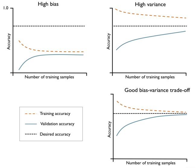
Debugging algorithms with learning curves
Diagnosing bias and variance problems with learning curves
Image(filename='images/06_04.png', width=600)
import matplotlib.pyplot as plt
from sklearn.model_selection import learning_curve


pipe_lr = make_pipeline(StandardScaler(),
                        LogisticRegression(penalty='l2', random_state=1))

train_sizes, train_scores, test_scores =\
                learning_curve(estimator=pipe_lr,
                               X=X_train,
                               y=y_train,
                               train_sizes=np.linspace(0.1, 1.0, 10),
                               cv=10,
                               n_jobs=1)

train_mean = np.mean(train_scores, axis=1)
train_std = np.std(train_scores, axis=1)
test_mean = np.mean(test_scores, axis=1)
test_std = np.std(test_scores, axis=1)

plt.plot(train_sizes, train_mean,
         color='blue', marker='o',
         markersize=5, label='training accuracy')

plt.fill_between(train_sizes,
                 train_mean + train_std,
                 train_mean - train_std,
                 alpha=0.15, color='blue')

plt.plot(train_sizes, test_mean,
         color='green', linestyle='--',
         marker='s', markersize=5,
         label='validation accuracy')

plt.fill_between(train_sizes,
                 test_mean + test_std,
                 test_mean - test_std,
                 alpha=0.15, color='green')

plt.grid()
plt.xlabel('Number of training samples')
plt.ylabel('Accuracy')
plt.legend(loc='lower right')
plt.ylim([0.8, 1.03])
plt.tight_layout()
#plt.savefig('images/06_05.png', dpi=300)
plt.show()

Addressing over- and underfitting with validation curves
from sklearn.model_selection import validation_curve


param_range = [0.001, 0.01, 0.1, 1.0, 10.0, 100.0]
train_scores, test_scores = validation_curve(
                estimator=pipe_lr,
                X=X_train,
                y=y_train,
                param_name='logisticregression__C',
                param_range=param_range,
                cv=10)

train_mean = np.mean(train_scores, axis=1)
train_std = np.std(train_scores, axis=1)
test_mean = np.mean(test_scores, axis=1)
test_std = np.std(test_scores, axis=1)

plt.plot(param_range, train_mean,
         color='blue', marker='o',
         markersize=5, label='training accuracy')

plt.fill_between(param_range, train_mean + train_std,
                 train_mean - train_std, alpha=0.15,
                 color='blue')

plt.plot(param_range, test_mean,
         color='green', linestyle='--',
         marker='s', markersize=5,
         label='validation accuracy')

plt.fill_between(param_range,
                 test_mean + test_std,
                 test_mean - test_std,
                 alpha=0.15, color='green')

plt.grid()
plt.xscale('log')
plt.legend(loc='lower right')
plt.xlabel('Parameter C')
plt.ylabel('Accuracy')
plt.ylim([0.8, 1.0])
plt.tight_layout()
# plt.savefig('images/06_06.png', dpi=300)
plt.show()

Fine-tuning machine learning models via grid search
Tuning hyperparameters via grid search
from sklearn.model_selection import GridSearchCV
from sklearn.svm import SVC

pipe_svc = make_pipeline(StandardScaler(),
                         SVC(random_state=1))

param_range = [0.0001, 0.001, 0.01, 0.1, 1.0, 10.0, 100.0, 1000.0]

param_grid = [{'svc__C': param_range,
               'svc__kernel': ['linear']},
              {'svc__C': param_range,
               'svc__gamma': param_range,
               'svc__kernel': ['rbf']}]

gs = GridSearchCV(estimator=pipe_svc,
                  param_grid=param_grid,
                  scoring='accuracy',
                  cv=10,
                  n_jobs=-1)
gs = gs.fit(X_train, y_train)
print(gs.best_score_)
print(gs.best_params_)
0.984615384615
{'svc__C': 100.0, 'svc__gamma': 0.001, 'svc__kernel': 'rbf'}
clf = gs.best_estimator_
clf.fit(X_train, y_train)
print('Test accuracy: %.3f' % clf.score(X_test, y_test))
Test accuracy: 0.974
Algorithm selection with nested cross-validation
Image(filename='images/06_07.png', width=500)

gs = GridSearchCV(estimator=pipe_svc,
                  param_grid=param_grid,
                  scoring='accuracy',
                  cv=2)

scores = cross_val_score(gs, X_train, y_train,
                         scoring='accuracy', cv=5)
print('CV accuracy: %.3f +/- %.3f' % (np.mean(scores),
                                      np.std(scores)))
CV accuracy: 0.974 +/- 0.015
from sklearn.tree import DecisionTreeClassifier

gs = GridSearchCV(estimator=DecisionTreeClassifier(random_state=0),
                  param_grid=[{'max_depth': [1, 2, 3, 4, 5, 6, 7, None]}],
                  scoring='accuracy',
                  cv=2)

scores = cross_val_score(gs, X_train, y_train,
                         scoring='accuracy', cv=5)
print('CV accuracy: %.3f +/- %.3f' % (np.mean(scores),
                                      np.std(scores)))
CV accuracy: 0.934 +/- 0.016
Looking at different performance evaluation metrics
…
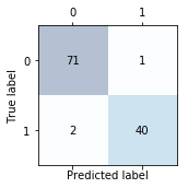
Reading a confusion matrix
Image(filename='images/06_08.png', width=300)

from sklearn.metrics import confusion_matrix

pipe_svc.fit(X_train, y_train)
y_pred = pipe_svc.predict(X_test)
confmat = confusion_matrix(y_true=y_test, y_pred=y_pred)
print(confmat)
[[71  1]
 [ 2 40]]
fig, ax = plt.subplots(figsize=(2.5, 2.5))
ax.matshow(confmat, cmap=plt.cm.Blues, alpha=0.3)
for i in range(confmat.shape[0]):
    for j in range(confmat.shape[1]):
        ax.text(x=j, y=i, s=confmat[i, j], va='center', ha='center')

plt.xlabel('Predicted label')
plt.ylabel('True label')

plt.tight_layout()
#plt.savefig('images/06_09.png', dpi=300)
plt.show()
Additional Note
Remember that we previously encoded the class labels so that malignant samples are the “postive” class (1), and benign samples are the “negative” class (0):
le.transform(['M', 'B'])
array([1, 0])
confmat = confusion_matrix(y_true=y_test, y_pred=y_pred)
print(confmat)
[[71  1]
 [ 2 40]]
Next, we printed the confusion matrix like so:
confmat = confusion_matrix(y_true=y_test, y_pred=y_pred)
print(confmat)
[[71  1]
 [ 2 40]]
Note that the (true) class 0 samples that are correctly predicted as class 0 (true negatives) are now in the upper left corner of the matrix (index 0, 0). In order to change the ordering so that the true negatives are in the lower right corner (index 1,1) and the true positves are in the upper left, we can use the labels argument like shown below:
confmat = confusion_matrix(y_true=y_test, y_pred=y_pred, labels=[1, 0])
print(confmat)
[[40  2]
 [ 1 71]]
We conclude:
Assuming that class 1 (malignant) is the positive class in this example, our model correctly classified 71 of the samples that belong to class 0 (true negatives) and 40 samples that belong to class 1 (true positives), respectively. However, our model also incorrectly misclassified 1 sample from class 0 as class 1 (false positive), and it predicted that 2 samples are benign although it is a malignant tumor (false negatives).
Optimizing the precision and recall of a classification model
from sklearn.metrics import precision_score, recall_score, f1_score

print('Precision: %.3f' % precision_score(y_true=y_test, y_pred=y_pred))
print('Recall: %.3f' % recall_score(y_true=y_test, y_pred=y_pred))
print('F1: %.3f' % f1_score(y_true=y_test, y_pred=y_pred))
Precision: 0.976
Recall: 0.952
F1: 0.964
from sklearn.metrics import make_scorer

scorer = make_scorer(f1_score, pos_label=0)

c_gamma_range = [0.01, 0.1, 1.0, 10.0]

param_grid = [{'svc__C': c_gamma_range,
               'svc__kernel': ['linear']},
              {'svc__C': c_gamma_range,
               'svc__gamma': c_gamma_range,
               'svc__kernel': ['rbf']}]

gs = GridSearchCV(estimator=pipe_svc,
                  param_grid=param_grid,
                  scoring=scorer,
                  cv=10,
                  n_jobs=-1)
gs = gs.fit(X_train, y_train)
print(gs.best_score_)
print(gs.best_params_)
0.986202145696
{'svc__C': 10.0, 'svc__gamma': 0.01, 'svc__kernel': 'rbf'}
Plotting a receiver operating characteristic
from sklearn.metrics import roc_curve, auc
from scipy import interp

pipe_lr = make_pipeline(StandardScaler(),
                        PCA(n_components=2),
                        LogisticRegression(penalty='l2',
                                           random_state=1,
                                           C=100.0))

X_train2 = X_train[:, [4, 14]]


cv = list(StratifiedKFold(n_splits=3,
                          random_state=1).split(X_train, y_train))

fig = plt.figure(figsize=(7, 5))

mean_tpr = 0.0
mean_fpr = np.linspace(0, 1, 100)
all_tpr = []

for i, (train, test) in enumerate(cv):
    probas = pipe_lr.fit(X_train2[train],
                         y_train[train]).predict_proba(X_train2[test])

    fpr, tpr, thresholds = roc_curve(y_train[test],
                                     probas[:, 1],
                                     pos_label=1)
    mean_tpr += interp(mean_fpr, fpr, tpr)
    mean_tpr[0] = 0.0
    roc_auc = auc(fpr, tpr)
    plt.plot(fpr,
             tpr,
             label='ROC fold %d (area = %0.2f)'
                   % (i+1, roc_auc))

plt.plot([0, 1],
         [0, 1],
         linestyle='--',
         color=(0.6, 0.6, 0.6),
         label='random guessing')

mean_tpr /= len(cv)
mean_tpr[-1] = 1.0
mean_auc = auc(mean_fpr, mean_tpr)
plt.plot(mean_fpr, mean_tpr, 'k--',
         label='mean ROC (area = %0.2f)' % mean_auc, lw=2)
plt.plot([0, 0, 1],
         [0, 1, 1],
         linestyle=':',
         color='black',
         label='perfect performance')

plt.xlim([-0.05, 1.05])
plt.ylim([-0.05, 1.05])
plt.xlabel('false positive rate')
plt.ylabel('true positive rate')
plt.legend(loc="lower right")

plt.tight_layout()
# plt.savefig('images/06_10.png', dpi=300)
plt.show()

[外链图片转存失败,源站可能有防盗链机制,建议将图片保存下来直接上传(img-YrmUwcEq-1586754580448)(output_76_0.png)]
The scoring metrics for multiclass classification
pre_scorer = make_scorer(score_func=precision_score,
                         pos_label=1,
                         greater_is_better=True,
                         average='micro')
Dealing with class imbalance
X_imb = np.vstack((X[y == 0], X[y == 1][:40]))
y_imb = np.hstack((y[y == 0], y[y == 1][:40]))
y_pred = np.zeros(y_imb.shape[0])
np.mean(y_pred == y_imb) * 100
89.924433249370267
from sklearn.utils import resample

print('Number of class 1 samples before:', X_imb[y_imb == 1].shape[0])

X_upsampled, y_upsampled = resample(X_imb[y_imb == 1],
                                    y_imb[y_imb == 1],
                                    replace=True,
                                    n_samples=X_imb[y_imb == 0].shape[0],
                                    random_state=123)

print('Number of class 1 samples after:', X_upsampled.shape[0])
Number of class 1 samples before: 40
Number of class 1 samples after: 357
X_bal = np.vstack((X[y == 0], X_upsampled))
y_bal = np.hstack((y[y == 0], y_upsampled))
y_pred = np.zeros(y_bal.shape[0])
np.mean(y_pred == y_bal) * 100
50.0
Summary
…
Readers may ignore the next cell.
! python ../.convert_notebook_to_script.py --input ch06.ipynb --output ch06.py
[NbConvertApp] Converting notebook ch06.ipynb to script
[NbConvertApp] Writing 16984 bytes to ch06.py