吴恩达机器学习CS229A_EX1_线性回归_Python3

单变量回归

问题描述：你的数据集中，x 是某个城市的人口数量，y 是你的餐车在那个城市的盈亏数额。对这个数据集进行挖掘，帮助你进行决策。

---

首先导入并分析数据：

import numpy as np
import pandas as pd
import matplotlib.pyplot as plt

def loadData(firename):
    return pd.read_csv(firename, header=None, names=['Population', 'Profit'])

data = loadData('ex1data1.txt')
print(data.head())
print(data.describe())
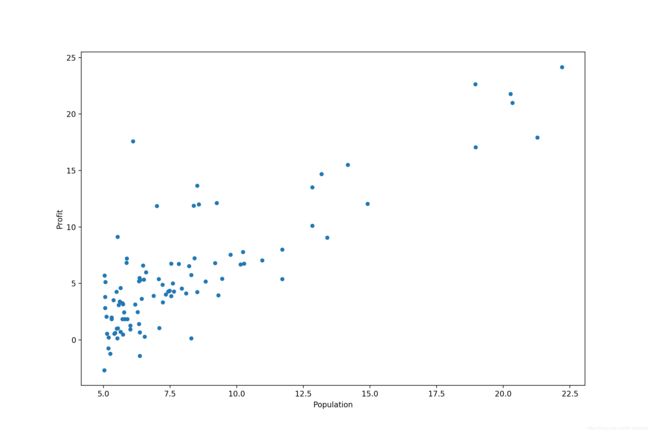
data.plot(kind='scatter', x='Population', y='Profit', figsize=(12, 8))
plt.show()

输出得到 data 的数据形式以及数据特征：

   Population   Profit
0      6.1101  17.5920
1      5.5277   9.1302
2      8.5186  13.6620
3      7.0032  11.8540
4      5.8598   6.8233

       Population     Profit
count   97.000000  97.000000
mean     8.159800   5.839135
std      3.869884   5.510262
min      5.026900  -2.680700
25%      5.707700   1.986900
50%      6.589400   4.562300
75%      8.578100   7.046700
max     22.203000  24.147000

Process finished with exit code 0

绘制数据集的散点图：

---

接着对数据进行预处理：

def initData(data):
    # 为每个样本添加 x0 = 1
    # 将数据集分为特征集和标签集
    data.insert(0, 'Ones', 1)
    cols = data.shape[1]
    X = data.iloc[:, 0:cols - 1]
    y = data.iloc[:, cols - 1:cols]
    # 将特征集和标签集转化为 numpy 矩阵
    X = np.matrix(X.values)
    y = np.matrix(y.values)
    # 初始化 alpha 为全 0
    theta = np.matrix(np.array([0, 0]))
    return X, y, theta

首先将 X 、y 分别转化为：

    Ones  Population
0      1      6.1101
1      1      5.5277
2      1      8.5186
3      1      7.0032
4      1      5.8598
..   ...         ...
92     1      5.8707
93     1      5.3054
94     1      8.2934
95     1     13.3940
96     1      5.4369

[97 rows x 2 columns]

      Profit
0   17.59200
1    9.13020
2   13.66200
3   11.85400
4    6.82330
..       ...
92   7.20290
93   1.98690
94   0.14454
95   9.05510
96   0.61705

[97 rows x 1 columns]

然后转化为 Numpy 矩阵，返回用于矩阵运算的 X 、y 、theta，可以查看三个矩阵的大小：

data = loadData('ex1data1.txt')
X, y, theta = initData(data)
print(X.shape, theta.shape, y.shape)

(97, 2) (1, 2) (97, 1)

Process finished with exit code 0

---

根据如下公式计算 cost ：

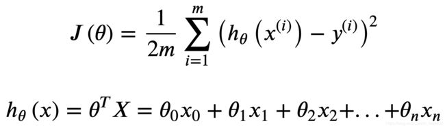
# 对给定 theta 计算 cost
def computeCost(X, y, theta):
    inner = np.power(((X * theta.T) - y), 2)
    return np.sum(inner) / (2 * len(X))

根据如下公式执行梯度下降算法：

# 梯度下降算法
# 需设定 alpha —— 学习率、 iters —— 迭代次数
def gradientDescent(X, y, theta, alpha, iters):
    # temp 用于缓存要更改的 theta
    temp = np.matrix(np.zeros(theta.shape))
    # theta 的元素个数
    parameters = int(theta.ravel().shape[1])
    # 初始化 cost 数组
    cost = np.zeros(iters)
    # 在设定的迭代次数内
    for i in range(iters):
        error = (X * theta.T) - y
        # 计算 theta j 要更改的值，保存在 temp 中
        for j in range(parameters):
            term = np.multiply(error, X[:, j])
            temp[0, j] = theta[0, j] - ((alpha / len(X)) * np.sum(term))
        # 更新 theta
        theta = temp
        # 计算并保存当前的 cost
        cost[i] = computeCost(X, y, theta)
    # 返回
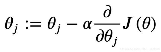
    return theta, cost

---

设置 alpha 为 0.01，iters 为 1000，运行并绘图：

alpha = 0.01
iters = 1000
data = loadData('ex1data1.txt')
X, y, theta = initData(data)
g, cost = gradientDescent(X, y, theta, alpha, iters)
print(g)

x = np.linspace(data.Population.min(), data.Population.max(), 100)
f = g[0, 0] + (g[0, 1] * x)

fig, ax = plt.subplots(figsize=(12,8))
ax.plot(x, f, 'r', label='Prediction')
ax.scatter(data.Population, data.Profit, label='Traning Data')
ax.legend(loc=2)
ax.set_xlabel('Population')
ax.set_ylabel('Profit')
ax.set_title('Predicted Profit vs. Population Size')
plt.show()

[[-3.24140214  1.1272942 ]]

Process finished with exit code 0

---

绘制 cost - iters 图像：

alpha = 0.01
iters = 1000
data = loadData('ex1data1.txt')
X, y, theta = initData(data)
g, cost = gradientDescent(X, y, theta, alpha, iters)
print(g)
fig, ax = plt.subplots(figsize=(12,8))
ax.plot(np.arange(iters), cost, 'r')
ax.set_xlabel('Iterations')
ax.set_ylabel('Cost')
ax.set_title('Error vs. Training Epoch')
plt.show()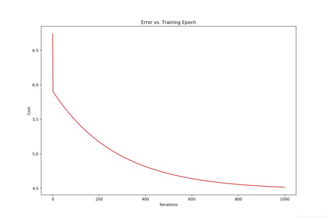

---

单变量回归完整程序：

import numpy as np
import pandas as pd
import matplotlib.pyplot as plt

def loadData(firename):
    return pd.read_csv(firename, header=None, names=['Population', 'Profit'])

def showData(data):
    data.plot(kind='scatter', x='Population', y='Profit', figsize=(12, 8))
    plt.show()

def initData(data):
    # 为每个样本添加 x0 = 1
    # 将数据集分为特征集和标签集
    data.insert(0, 'Ones', 1)
    cols = data.shape[1]
    X = data.iloc[:, 0:cols - 1]
    y = data.iloc[:, cols - 1:cols]
    # 将特征集和标签集转化为 numpy 矩阵
    X = np.matrix(X.values)
    y = np.matrix(y.values)
    # 初始化 alpha 为全 0
    theta = np.matrix(np.array([0, 0]))
    return X, y, theta

# 对给定 theta 计算 cost
def computeCost(X, y, theta):
    inner = np.power(((X * theta.T) - y), 2)
    return np.sum(inner) / (2 * len(X))

# 梯度下降算法
# 需设定 alpha —— 学习率、 iters —— 迭代次数
def gradientDescent(X, y, theta, alpha, iters):
    # temp 用于缓存要更改的 theta
    temp = np.matrix(np.zeros(theta.shape))
    # theta 的元素个数
    parameters = int(theta.ravel().shape[1])
    # 初始化 cost 数组
    cost = np.zeros(iters)
    # 在设定的迭代次数内
    for i in range(iters):
        error = (X * theta.T) - y
        # 计算 theta j 要更改的值，保存在 temp 中
        for j in range(parameters):
            term = np.multiply(error, X[:, j])
            temp[0, j] = theta[0, j] - ((alpha / len(X)) * np.sum(term))
        # 更新 theta
        theta = temp
        # 计算并保存当前的 cost
        cost[i] = computeCost(X, y, theta)
    # 返回
    return theta, cost

def showRegression(data, g):
    x = np.linspace(data.Population.min(), data.Population.max(), 100)
    f = g[0, 0] + (g[0, 1] * x)
    fig, ax = plt.subplots(figsize=(12, 8))
    ax.plot(x, f, 'r', label='Prediction')
    ax.scatter(data.Population, data.Profit, label='Traning Data')
    ax.legend(loc=2)
    ax.set_xlabel('Population')
    ax.set_ylabel('Profit')
    ax.set_title('Predicted Profit vs. Population Size')
    plt.show()

def showCost_Iters(iters, cost):
    fig, ax = plt.subplots(figsize=(12, 8))
    ax.plot(np.arange(iters), cost, 'r')
    ax.set_xlabel('Iterations')
    ax.set_ylabel('Cost')
    ax.set_title('Error vs. Training Epoch')
    plt.show()

alpha = 0.01
iters = 1000
data = loadData('ex1data1.txt')
X, y, theta = initData(data)
g, cost = gradientDescent(X, y, theta, alpha, iters)
print(g)

#showRegression(data, g)
#showCost_Iters(iters, cost)

---

---

多变量回归

问题描述：你的数据集中，x1 代表房屋面积、x2 代表卧室数量，y 代表售价。要求基于这个数据集训练一个预测房价的模型。

---

对单变量回归的完整函数稍作修改：

import numpy as np
import pandas as pd
import matplotlib.pyplot as plt

def loadData(firename):
    return pd.read_csv(firename, header=None, names=['Size', 'Bedrooms', 'Price'])

def initData(data):
    # 特征缩放
    data = (data - data.mean()) / data.std()
    # 为每个样本添加 x0 = 1
    # 将数据集分为特征集和标签集
    data.insert(0, 'Ones', 1)
    cols = data.shape[1]
    X = data.iloc[:, 0:cols - 1]
    y = data.iloc[:, cols - 1:cols]
    # 将特征集和标签集转化为 numpy 矩阵
    X = np.matrix(X.values)
    y = np.matrix(y.values)
    # 初始化 alpha 为全 0
    theta = np.matrix(np.array([0, 0, 0]))
    return X, y, theta

# 对给定 theta 计算 cost
def computeCost(X, y, theta):
    inner = np.power(((X * theta.T) - y), 2)
    return np.sum(inner) / (2 * len(X))

# 梯度下降算法
# 需设定 alpha —— 学习率、 iters —— 迭代次数
def gradientDescent(X, y, theta, alpha, iters):
    # temp 用于缓存要更改的 theta
    temp = np.matrix(np.zeros(theta.shape))
    # theta 的元素个数
    parameters = int(theta.ravel().shape[1])
    # 初始化 cost 数组
    cost = np.zeros(iters)
    # 在设定的迭代次数内
    for i in range(iters):
        error = (X * theta.T) - y
        # 计算 theta j 要更改的值，保存在 temp 中
        for j in range(parameters):
            term = np.multiply(error, X[:, j])
            temp[0, j] = theta[0, j] - ((alpha / len(X)) * np.sum(term))
        # 更新 theta
        theta = temp
        # 计算并保存当前的 cost
        cost[i] = computeCost(X, y, theta)
    # 返回
    return theta, cost

def showCost_Iters(iters, cost):
    fig, ax = plt.subplots(figsize=(12, 8))
    ax.plot(np.arange(iters), cost, 'r')
    ax.set_xlabel('Iterations')
    ax.set_ylabel('Cost')
    ax.set_title('Error vs. Training Epoch')
    plt.show()

alpha = 0.01
iters = 1000
data = loadData('ex1data2.txt')
X, y, theta = initData(data)
g, cost = gradientDescent(X, y, theta, alpha, iters)
print(g)

showCost_Iters(iters, cost)

[[-1.10868761e-16  8.78503652e-01 -4.69166570e-02]]

Process finished with exit code 0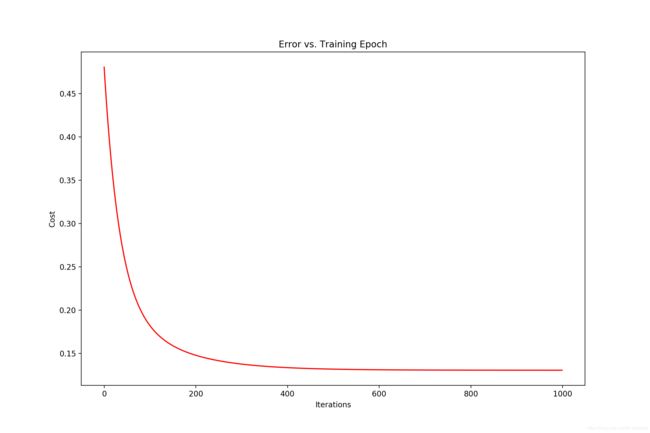

---

---

使用 Sklearn 库

以单变量回归为例

import numpy as np
import pandas as pd
import matplotlib.pyplot as plt
from sklearn import linear_model

def loadData(firename):
    return pd.read_csv(firename, header=None, names=['Population', 'Profit'])

def initData(data):
    # 为每个样本添加 x0 = 1
    # 将数据集分为特征集和标签集
    data.insert(0, 'Ones', 1)
    cols = data.shape[1]
    X = data.iloc[:, 0:cols - 1]
    y = data.iloc[:, cols - 1:cols]
    # 将特征集和标签集转化为 numpy 矩阵
    X = np.matrix(X.values)
    y = np.matrix(y.values)
    return X, y

def showRegression(X, model):
    x = np.array(X[:, 1].A1)
    f = model.predict(X).flatten()

    fig, ax = plt.subplots(figsize=(12, 8))
    ax.plot(x, f, 'r', label='Prediction')
    ax.scatter(data.Population, data.Profit, label='Traning Data')
    ax.legend(loc=2)
    ax.set_xlabel('Population')
    ax.set_ylabel('Profit')
    ax.set_title('Predicted Profit vs. Population Size')
    plt.show()


data = loadData('ex1data1.txt')
X, y = initData(data)
model = linear_model.LinearRegression()
model.fit(X, y)

showRegression(X, model)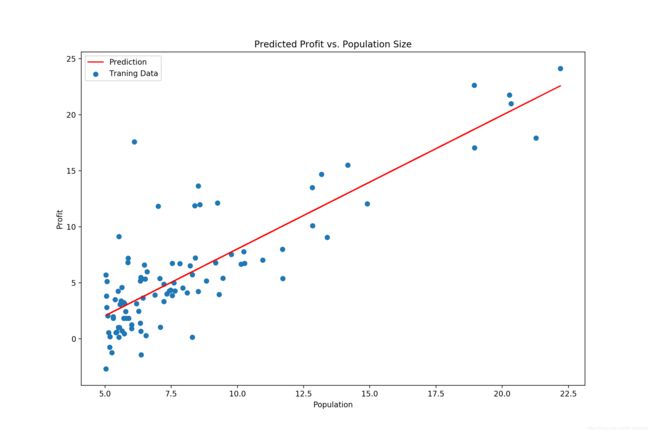

---

---

正规方程法

以单变量回归为例

import numpy as np
import pandas as pd

def loadData(firename):
    return pd.read_csv(firename, header=None, names=['Population', 'Profit'])

def initData(data):
    # 为每个样本添加 x0 = 1
    # 将数据集分为特征集和标签集
    data.insert(0, 'Ones', 1)
    cols = data.shape[1]
    X = data.iloc[:, 0:cols - 1]
    y = data.iloc[:, cols - 1:cols]
    # 将特征集和标签集转化为 numpy 矩阵
    X = np.matrix(X.values)
    y = np.matrix(y.values)
    return X, y

def normalEqn(X, y):
    # X.T@X 等价于 X.T.dot(X)
    theta = np.linalg.inv(X.T@X)@X.T@y
    return theta


data = loadData('ex1data1.txt')
X, y = initData(data)
theta = normalEqn(X, y)
print(theta)

[[-3.89578088]
 [ 1.19303364]]

Process finished with exit code 0