吴恩达机器学习CS229A_EX3_LR与NN手写数字识别_Python3

任务描述

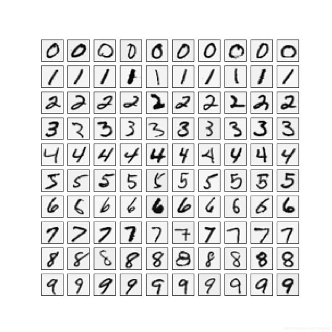
数据集为手写数字，是一个多分类问题，分别用逻辑回归和神经网络做。

---

逻辑回归

逻辑回归及其正则化已经在 EX 2 做过，这里做一些修改即可。

---

首先导入数据，给出的数据集是 Matlab 的 .mat 格式，每个样本是 20 * 20 的灰度图，共 5000 个样本：

import numpy as np
from scipy.io import loadmat
import scipy.optimize as opt

def loadData(filename):
    return loadmat(filename)

data = loadmat('ex3data1.mat')
print(data['X'].shape, data['y'].shape)

(5000, 400) (5000, 1)

Process finished with exit code 0

接着对数据预处理 ，因为是数字 0 ～ 9 的多分类问题，需要 10 个分类器，这里 theta 初始化为大小为 11 * n+1 的数组，11 是因为数字 0 的标签是 10，这样后续程序写起来比较简洁。

def initData(data):
    # 样本数
    m = data['X'].shape[0]
    # 特征数
    n = data['X'].shape[1]
    # 增加一列 bias
    data['X'] = np.append(data['X'], np.ones(m).reshape(m,1), axis=1)
    X = data['X']
    y = data['y']
    theta = np.zeros((11, n + 1))
    return X, y, theta

---

编写 Logistic Regression 需要的函数，详细内容可参考： 吴恩达机器学习CS229A_EX2_逻辑回归与正则化 。

这里根据要求对梯度求解函数做了改写，用矩阵运算替代循环，函数的计算结果和之前的是一样的。

def sigmoid(z):
    return 1 / (1 + np.exp(-z))

def costReg(theta, X, y, lamda):
    n = len(theta)
    m = len(y)
    first = -y * np.log(sigmoid(X @ theta.reshape(n,1)))
    second = -(1 - y) * np.log(1 - sigmoid(X @ theta.reshape(n,1)))
    reg = (lamda / (2 * m)) * np.sum(np.power(theta.reshape(n,1), 2))
    return (sum(first + second) / m) + reg

def gradientReg_noLoop(theta, X, y, lamda):
    n = len(theta)
    m = len(y)
    error = sigmoid(X @ theta.reshape(n, 1)) - y
    grad = (X.T @ error / m) + ((lamda / m) * theta.reshape(n, 1))
    grad[0][0] = np.sum(error * X[:, 0].reshape(m, 1)) / m
    grad = np.reshape(grad, (n,))
    return grad

---

编写分类函数和测试函数：

# 分类函数
def one_vs_all(theta, X, y, lamda):
    m = len(y)
    n = len(theta[0])
    # 从 1 到 10 总共训练 10 个分类器，依次保存到 theta
    for i in range(1, 11):
        # label 为 i 置 1，不为 i 置 0
        y_i = np.array([1 if label == i else 0 for label in y])
        y_i = np.reshape(y_i,(m, 1))
        theta_i = theta[i,:]
        theta_i = np.reshape(theta_i,(n, 1))
        # 使用 scipy 的库函数就算最优参数
        result = opt.fmin_tnc(func=costReg, x0=theta_i, fprime=gradientReg_noLoop, args=(X, y_i, lamda))
        # 保存第 i 个分类器
        theta[i,:] = result[0]

# 测试函数
def predict_all(theta, X, y):
    m = len(y)
    y_pre = np.zeros((m, 2))
    # term 为 m * 10 的数组，每一行依次记录该样本为 1，2，……，9，0 的概率
    term = sigmoid(X @ theta.T)
    # 选取最大概率对应的 label 作为预测结果
    for sample in range(m):
        for i in range(1, 11):
            if(term[sample][i] > y_pre[sample][1]):
                y_pre[sample][0] = i
                y_pre[sample][1] = term[sample][i]
    rate = 0.0
    for sample in range(m):
        if(y_pre[sample][0] == y[sample]):
            rate += 1
    rate = (rate / m) * 100
    print('accuracy = {0}%'.format(rate))

---

执行并测试，可以看到这里不做正则化限制效果更好 ：

data = loadData('ex3data1.mat')
X, y, theta = initData(data)
one_vs_all(theta, X, y, 0)
predict_all(theta, X, y)

accuracy = 97.36%

Process finished with exit code 0

data = loadData('ex3data1.mat')
X, y, theta = initData(data)
one_vs_all(theta, X, y, 0.1)
predict_all(theta, X, y)

accuracy = 96.5%

Process finished with exit code 0

data = loadData('ex3data1.mat')
X, y, theta = initData(data)
one_vs_all(theta, X, y, 1)
predict_all(theta, X, y)

accuracy = 94.39999999999999%

Process finished with exit code 0

---

完整程序：

import numpy as np
from scipy.io import loadmat
import scipy.optimize as opt

def loadData(filename):
    return loadmat(filename)

def initData(data):
    # 样本数
    m = data['X'].shape[0]
    # 特征数
    n = data['X'].shape[1]
    # 增加一列 bias
    data['X'] = np.append(data['X'], np.ones(m).reshape(m,1), axis=1)
    X = data['X']
    y = data['y']
    theta = np.zeros((11, n + 1))
    return X, y, theta

def sigmoid(z):
    return 1 / (1 + np.exp(-z))

def costReg(theta, X, y, lamda):
    n = len(theta)
    m = len(y)
    first = -y * np.log(sigmoid(X @ theta.reshape(n,1)))
    second = -(1 - y) * np.log(1 - sigmoid(X @ theta.reshape(n,1)))
    reg = (lamda / (2 * m)) * np.sum(np.power(theta.reshape(n,1), 2))
    return (sum(first + second) / m) + reg

def gradientReg_noLoop(theta, X, y, lamda):
    n = len(theta)
    m = len(y)
    error = sigmoid(X @ theta.reshape(n, 1)) - y
    grad = (X.T @ error / m) + ((lamda / m) * theta.reshape(n, 1))
    grad[0][0] = np.sum(error * X[:, 0].reshape(m, 1)) / m
    grad = np.reshape(grad, (n,))
    return grad

# 分类函数
def one_vs_all(theta, X, y, lamda):
    m = len(y)
    n = len(theta[0])
    # 从 1 到 10 总共训练 10 个分类器，依次保存到 theta
    for i in range(1, 11):
        # label 为 i 置 1，不为 i 置 0
        y_i = np.array([1 if label == i else 0 for label in y])
        y_i = np.reshape(y_i,(m, 1))
        theta_i = theta[i,:]
        theta_i = np.reshape(theta_i,(n, 1))
        # 使用 scipy 的库函数就算最优参数
        result = opt.fmin_tnc(func=costReg, x0=theta_i, fprime=gradientReg_noLoop, args=(X, y_i, lamda))
        # 保存第 i 个分类器
        theta[i,:] = result[0]

# 测试函数
def predict_all(theta, X, y):
    m = len(y)
    y_pre = np.zeros((m, 2))
    # term 为 m * 10 的数组，每一行依次记录该样本为 1，2，……，9，0 的概率
    term = sigmoid(X @ theta.T)
    # 选取最大概率对应的 label 作为预测结果
    for sample in range(m):
        for i in range(1, 11):
            if(term[sample][i] > y_pre[sample][1]):
                y_pre[sample][0] = i
                y_pre[sample][1] = term[sample][i]
    rate = 0.0
    for sample in range(m):
        if(y_pre[sample][0] == y[sample]):
            rate += 1
    rate = (rate / m) * 100
    print('accuracy = {0}%'.format(rate))


data = loadData('ex3data1.mat')
X, y, theta = initData(data)
one_vs_all(theta, X, y, 0)
predict_all(theta, X, y)

 

---

---

神经网络

这里神经网络的参数已经给出，不需要进行训练（下一个 EX 做），我们只需要编程写出神经网络的结构，执行分类就行。

---

导入并初始化数据：

import numpy as np
import matplotlib
import matplotlib.pyplot as plt
from scipy.io import loadmat

def loadData(filename):
    return loadmat(filename)

def initData(data):
    X = data['X']
    # X : 增加一列 bias（要增加到第一列）
    X = np.insert(X, 0, values=np.ones(X.shape[0]), axis=1)
    y = data['y']
    return X, y

data = loadData('ex3data1.mat')
X, y = initData(data)
print(X.shape, y.shape)
theta = loadData('ex3weights.mat')
theta1 = theta['Theta1']
theta2 = theta['Theta2']
print(theta1.shape, theta2.shape)

(5000, 401) (5000, 1)
(25, 401) (10, 26)

Process finished with exit code 0

 

---

根据神经网络的结构（一层输入层 400+1 ，一层隐藏层 25+1 ，一层输出层 10），计算结果： 

def sigmoid(z):
    return 1 / (1 + np.exp(-z))

def NN(X, theta1, theta2):
    hidden_layer = sigmoid(X @ theta1.T)
    hidden_layer = np.insert(hidden_layer, 0, values=np.ones(X.shape[0]), axis=1)
    output = sigmoid(hidden_layer @ theta2.T)
    return output

---

测试结果，正确率 97.52% ：

def predict(output, y):
    m = len(y)
    rate = 0.0
    for sample in range(m):
        pre_res = -1
        pre_pro = 0.0
        for i in range(10):
            if(output[sample][i] > pre_pro):
                pre_res = i + 1
                pre_pro = output[sample][i]
        if(pre_res == y[sample]):
            rate += 1
        print(pre_res)
    rate = (rate / m) * 100
    print('accuracy = {0}%'.format(rate))


data = loadData('ex3data1.mat')
X, y = initData(data)
theta = loadData('ex3weights.mat')
theta1 = theta['Theta1']
theta2 = theta['Theta2']
output = NN(X, theta1, theta2)
predict(output, y)

accuracy = 97.52%

Process finished with exit code 0

---

这里笔者试着可视化隐藏层，看看能否观察出什么：

 找了 100 个样本，在对应位置打印它们在隐藏层的 5*5 的图像：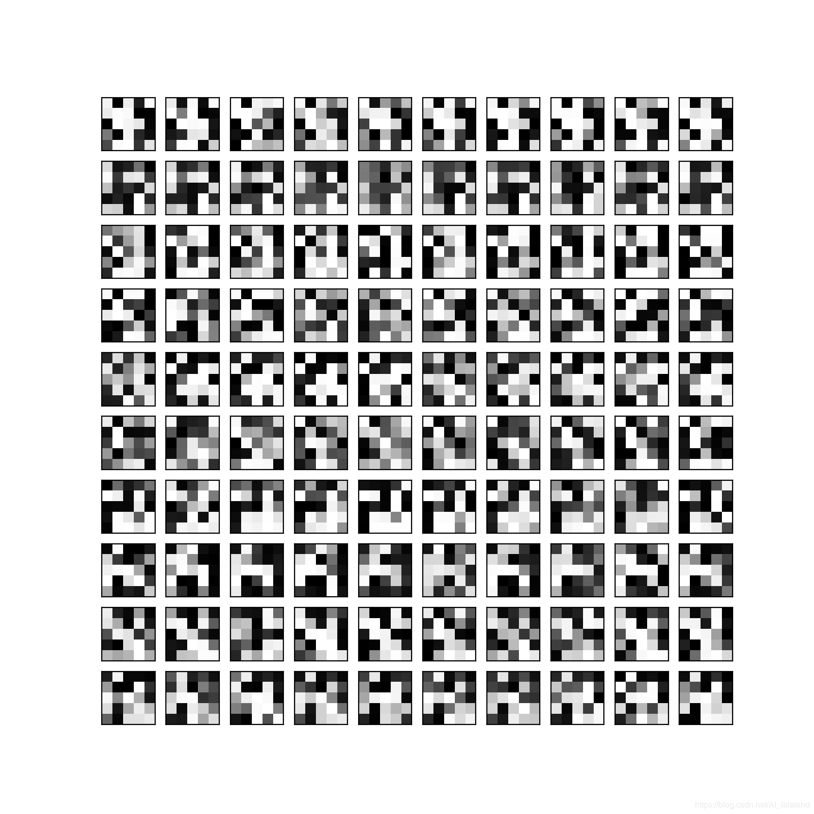

果然并不能观察出什么。。。

---

完整程序：

import numpy as np
import matplotlib
import matplotlib.pyplot as plt
from scipy.io import loadmat

def loadData(filename):
    return loadmat(filename)

def initData(data):
    X = data['X']
    # X : 增加一列 bias（要增加到第一列）
    X = np.insert(X, 0, values=np.ones(X.shape[0]), axis=1)
    y = data['y']
    return X, y

def sigmoid(z):
    return 1 / (1 + np.exp(-z))

def NN(X, theta1, theta2):
    hidden_layer = sigmoid(X @ theta1.T)
    hidden_layer = np.insert(hidden_layer, 0, values=np.ones(X.shape[0]), axis=1)
    output = sigmoid(hidden_layer @ theta2.T)
    return output

def predict(output, y):
    m = len(y)
    rate = 0.0
    for sample in range(m):
        pre_res = -1
        pre_pro = 0.0
        for i in range(10):
            if(output[sample][i] > pre_pro):
                pre_res = i + 1
                pre_pro = output[sample][i]
        if(pre_res == y[sample]):
            rate += 1
        print(pre_res)
    rate = (rate / m) * 100
    print('accuracy = {0}%'.format(rate))

def visualizing(layer):
    sample_idx = range(0,5000,50)
    sample_images = layer[sample_idx, :]
    fig, ax_array = plt.subplots(nrows=10, ncols=10, sharey=True, sharex=True, figsize=(8, 8))
    for r in range(10):
        for c in range(10):
            ax_array[r, c].matshow(sample_images[10 * r + c].reshape((5, 5)).T,cmap=matplotlib.cm.binary)
            plt.xticks(np.array([]))
            plt.yticks(np.array([]))
    plt.show()


data = loadData('ex3data1.mat')
X, y = initData(data)
theta = loadData('ex3weights.mat')
theta1 = theta['Theta1']
theta2 = theta['Theta2']
output = NN(X, theta1, theta2)
predict(output, y)